Introduction and Guidelines

This page provides a brief introduction to graph matching and some guidelines for using pygmtools. If you are seeking some background information, this is the right place!

Note

For more technical details, we recommend the following two surveys.

About learning-based deep graph matching: Junchi Yan, Shuang Yang, Edwin Hancock. “Learning Graph Matching and Related Combinatorial Optimization Problems.” IJCAI 2020.

About non-learning two-graph matching and multi-graph matching: Junchi Yan, Xu-Cheng Yin, Weiyao Lin, Cheng Deng, Hongyuan Zha, Xiaokang Yang. “A Short Survey of Recent Advances in Graph Matching.” ICMR 2016.

Why Graph Matching?

Graph Matching (GM) is a fundamental yet challenging problem in pattern recognition, data mining, and others. GM aims to find node-to-node correspondence among multiple graphs, by solving an NP-hard combinatorial problem. Recently, there is growing interest in developing deep learning-based graph matching methods.

Compared to other straight-forward matching methods e.g. greedy matching, graph matching methods are more reliable because it is based on an optimization form. Besides, graph matching methods exploit both node affinity and edge affinity, thus graph matching methods are usually more robust to noises and outliers. The recent line of deep graph matching methods also enables many graph matching solvers to be integrated into a deep learning pipeline.

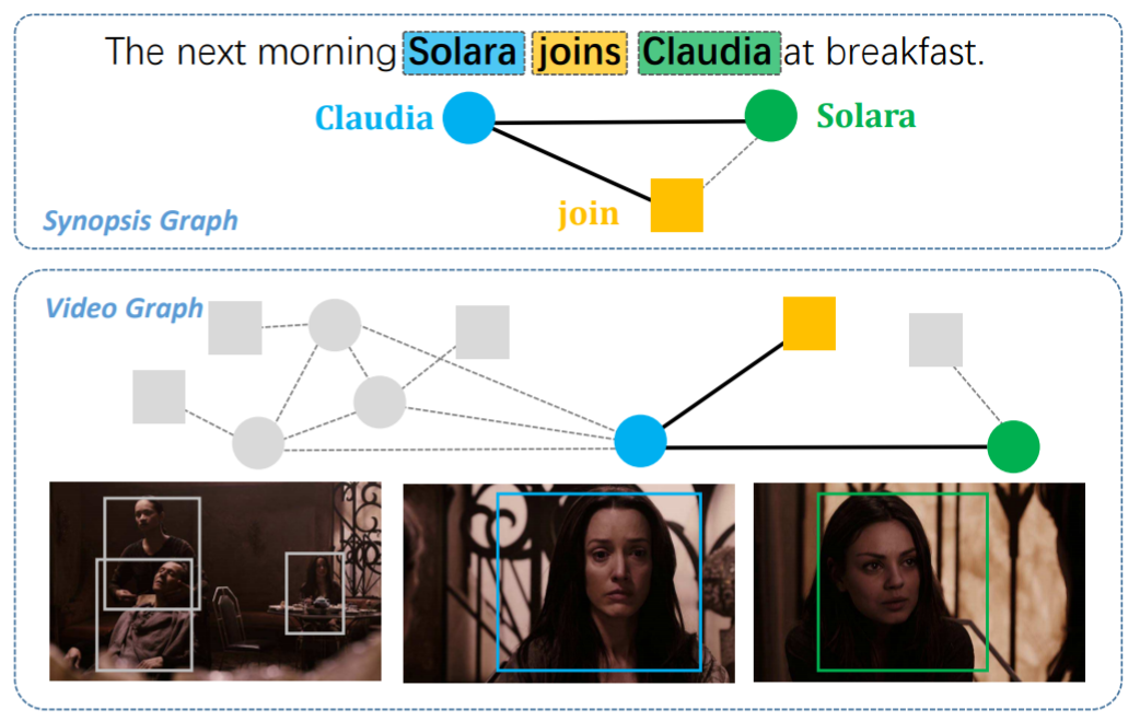
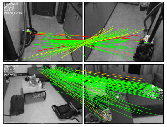
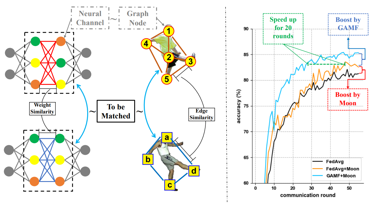
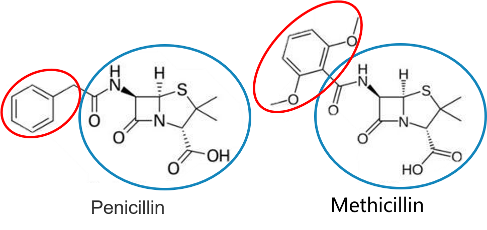
Graph matching techniques have been applied to the following applications:

• Bridging movie and synopses

  

• Image correspondence

  

• Model ensemble and federated learning

  

• Molecules matching

  

• and more…

If your task involves matching two or more graphs, you should try the solvers in pygmtools!

What is Graph Matching?

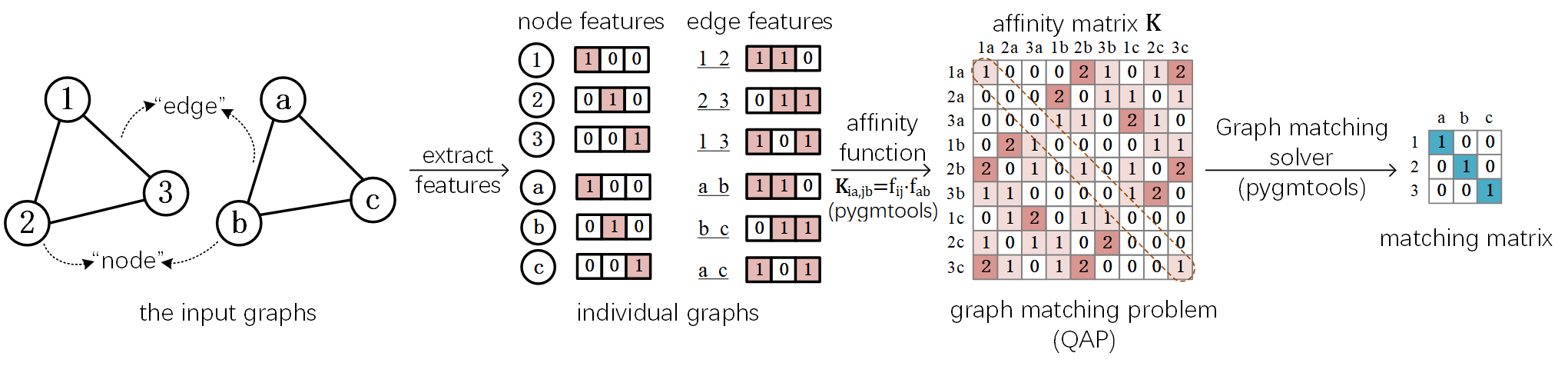
The Graph Matching Pipeline

Solving a real-world graph-matching problem may involve the following steps:

1. Extract node/edge features from the graphs you want to match.

2. Build an affinity matrix from node/edge features.

3. Solve the graph matching problem with GM solvers.

And Step 1 may be done by methods depending on your application, Step 2&3 can be handled by pygmtools. The following plot illustrates a standard deep graph matching pipeline.

The Math Form

Let’s involve a little bit of math to better understand the graph matching pipeline. In general, graph matching is of the following form, known as Quadratic Assignment Problem (QAP):

\[\begin{split}&\max_{\mathbf{X}} \ \texttt{vec}(\mathbf{X})^\top \mathbf{K} \texttt{vec}(\mathbf{X})\\ s.t. \quad &\mathbf{X} \in \{0, 1\}^{n_1\times n_2}, \ \mathbf{X}\mathbf{1} = \mathbf{1}, \ \mathbf{X}^\top\mathbf{1} \leq \mathbf{1}\end{split}\]

The notations are explained as follows:

• \(\mathbf{X}\) is known as the permutation matrix which encodes the matching result. It is also the decision variable in graph matching problem. \(\mathbf{X}_{i,a}=1\) means node \(i\) in graph 1 is matched to node \(a\) in graph 2, and \(\mathbf{X}_{i,a}=0\) means non-matched. Without loss of generality, it is assumed that \(n_1\leq n_2.\) \(\mathbf{X}\) has the following constraints:

  • The sum of each row must be equal to 1: \(\mathbf{X}\mathbf{1} = \mathbf{1}\);

  • The sum of each column must be equal to, or smaller than 1: \(\mathbf{X}\mathbf{1} \leq \mathbf{1}\).

• \(\mathtt{vec}(\mathbf{X})\) means the column-wise vectorization form of \(\mathbf{X}\).

• \(\mathbf{1}\) means a column vector whose elements are all 1s.

• \(\mathbf{K}\) is known as the affinity matrix which encodes the information of the input graphs. Both node-wise and edge-wise affinities are encoded in \(\mathbf{K}\):

  • The diagonal element \(\mathbf{K}_{i + a\times n_1, i + a\times n_1}\) means the node-wise affinity of node \(i\) in graph 1 and node \(a\) in graph 2;

  • The off-diagonal element \(\mathbf{K}_{i + a\times n_1, j + b\times n_1}\) means the edge-wise affinity of edge \(ij\) in graph 1 and edge \(ab\) in graph 2.

Graph Matching Best Practice

We need to understand the advantages and limitations of graph matching solvers. As discussed above, the major advantage of graph matching solvers is that they are more robust to noises and outliers. Graph matching also utilizes edge information, which is usually ignored in linear matching methods. The major drawback of graph matching solvers is their efficiency and scalability since the optimization problem is NP-hard. Therefore, to decide which matching method is most suitable, one needs to balance between the required matching accuracy and the affordable time and memory cost according to his/her application.

Note

Anyway, it does no harm to try graph matching first!

When to use pygmtools

pygmtools is recommended for the following cases, and you could benefit from the friendly API:

• If you want to integrate graph matching as a step of your pipeline (either learning or non-learning).

• If you want a quick benchmarking and profiling of the graph matching solvers available in pygmtools.

• If you do not want to dive too deep into the algorithm details and do not need to modify the algorithm.

We offer the following guidelines for your reference:

• If you want to integrate graph matching solvers into your end-to-end supervised deep learning pipeline, try neural_solvers.

• If no ground truth label is available for the matching step, try classic_solvers.

• If there are multiple graphs to be jointly matched, try multi_graph_solvers.

• If time and memory cost of the above methods are unacceptable for your task, try linear_solvers.

When not to use pygmtools

As a highly packed toolkit, pygmtools lacks some flexibilities in the implementation details, especially for experts in graph matching. If you are researching new graph matching algorithms or developing next-generation deep graph matching neural networks, pygmtools may not be suitable. We recommend ThinkMatch as the protocol for academic research.