Note
Go to the end to download the full example code
Jittor Backend Example: Matching Image Keypoints by Graph Matching Neural Networks
This example shows how to match image keypoints by neural network-based graph matching solvers. These graph matching solvers are designed to match two individual graphs. The matched images can be further passed to tackle downstream tasks.
# Author: Runzhong Wang <runzhong.wang@sjtu.edu.cn>
#         Wenzheng Pan <pwz1121@sjtu.edu.cn>
#
# License: Mulan PSL v2 License
Note
The following solvers are based on matching two individual graphs, and are included in this example:
import jittor as jt # jittor backend
from jittor import Var, models, nn
import pygmtools as pygm
import matplotlib.pyplot as plt # for plotting
from matplotlib.patches import ConnectionPatch # for plotting matching result
import scipy.io as sio # for loading .mat file
import scipy.spatial as spa # for Delaunay triangulation
from sklearn.decomposition import PCA as PCAdimReduc
import itertools
import numpy as np
from PIL import Image
pygm.set_backend('jittor') # set default backend for pygmtools
Predicting Matching by Graph Matching Neural Networks
In this section we show how to do predictions (inference) by graph matching neural networks.
Let’s take PCA-GM (pca_gm()) as an example.
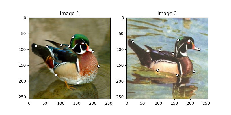
Load the images
Images are from the Willow Object Class dataset (this dataset also available with the Benchmark of pygmtools,
see WillowObject).
The images are resized to 256x256.
obj_resize = (256, 256)
img1 = Image.open('../data/willow_duck_0001.png')
img2 = Image.open('../data/willow_duck_0002.png')
kpts1 = jt.Var(sio.loadmat('../data/willow_duck_0001.mat')['pts_coord'])
kpts2 = jt.Var(sio.loadmat('../data/willow_duck_0002.mat')['pts_coord'])
kpts1[0] = kpts1[0] * obj_resize[0] / img1.size[0]
kpts1[1] = kpts1[1] * obj_resize[1] / img1.size[1]
kpts2[0] = kpts2[0] * obj_resize[0] / img2.size[0]
kpts2[1] = kpts2[1] * obj_resize[1] / img2.size[1]
img1 = img1.resize(obj_resize, resample=Image.BILINEAR)
img2 = img2.resize(obj_resize, resample=Image.BILINEAR)
jittor_img1 = jt.Var(np.array(img1, dtype=np.float32) / 256).permute(2, 0, 1).unsqueeze(0) # shape: BxCxHxW
jittor_img2 = jt.Var(np.array(img2, dtype=np.float32) / 256).permute(2, 0, 1).unsqueeze(0) # shape: BxCxHxW
Visualize the images and keypoints
def plot_image_with_graph(img, kpt, A=None):
    plt.imshow(img)
    plt.scatter(kpt[0], kpt[1], c='w', edgecolors='k')
    if A is not None:
        for idx in jt.nonzero(A):
            plt.plot((kpt[0, idx[0]], kpt[0, idx[1]]), (kpt[1, idx[0]], kpt[1, idx[1]]), 'k-')

plt.figure(figsize=(8, 4))
plt.subplot(1, 2, 1)
plt.title('Image 1')
plot_image_with_graph(img1, kpts1)
plt.subplot(1, 2, 2)
plt.title('Image 2')
plot_image_with_graph(img2, kpts2)
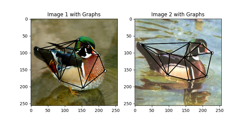
Build the graphs
Graph structures are built based on the geometric structure of the keypoint set. In this example, we refer to Delaunay triangulation.
def delaunay_triangulation(kpt):
    d = spa.Delaunay(kpt.numpy().transpose())
    A = jt.zeros((len(kpt[0]), len(kpt[0])))
    for simplex in d.simplices:
        for pair in itertools.permutations(simplex, 2):
            A[pair] = 1
    return A

A1 = delaunay_triangulation(kpts1)
A2 = delaunay_triangulation(kpts2)
Visualize the graphs
plt.figure(figsize=(8, 4))
plt.subplot(1, 2, 1)
plt.title('Image 1 with Graphs')
plot_image_with_graph(img1, kpts1, A1)
plt.subplot(1, 2, 2)
plt.title('Image 2 with Graphs')
plot_image_with_graph(img2, kpts2, A2)
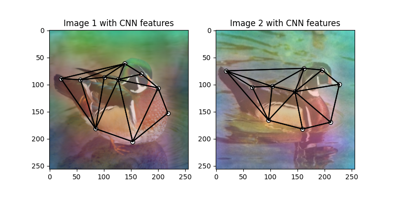
Extract node features via CNN
Deep graph matching solvers can be fused with CNN feature extractors, to build an end-to-end learning pipeline.
In this example, let’s adopt the deep graph solvers based on matching two individual graphs.
The image features are based on two intermediate layers from the VGG16 CNN model, following
existing deep graph matching papers (such as pca_gm())
Let’s firstly fetch and download the VGG16 model:
vgg16_cnn = models.vgg16_bn(True)
List of layers of VGG16:
print(vgg16_cnn.features)
Sequential(
    0: Conv(3, 64, (3, 3), (1, 1), (1, 1), (1, 1), 1, float32[64,], None, Kw=None, fan=None, i=None, bound=None)
    1: BatchNorm(64, 1e-05, momentum=0.1, affine=True, is_train=True, sync=True)
    2: relu()
    3: Conv(64, 64, (3, 3), (1, 1), (1, 1), (1, 1), 1, float32[64,], None, Kw=None, fan=None, i=None, bound=None)
    4: BatchNorm(64, 1e-05, momentum=0.1, affine=True, is_train=True, sync=True)
    5: relu()
    6: Pool((2, 2), (2, 2), padding=(0, 0), dilation=None, return_indices=None, ceil_mode=False, count_include_pad=False, op=maximum)
    7: Conv(64, 128, (3, 3), (1, 1), (1, 1), (1, 1), 1, float32[128,], None, Kw=None, fan=None, i=None, bound=None)
    8: BatchNorm(128, 1e-05, momentum=0.1, affine=True, is_train=True, sync=True)
    9: relu()
    10: Conv(128, 128, (3, 3), (1, 1), (1, 1), (1, 1), 1, float32[128,], None, Kw=None, fan=None, i=None, bound=None)
    11: BatchNorm(128, 1e-05, momentum=0.1, affine=True, is_train=True, sync=True)
    12: relu()
    13: Pool((2, 2), (2, 2), padding=(0, 0), dilation=None, return_indices=None, ceil_mode=False, count_include_pad=False, op=maximum)
    14: Conv(128, 256, (3, 3), (1, 1), (1, 1), (1, 1), 1, float32[256,], None, Kw=None, fan=None, i=None, bound=None)
    15: BatchNorm(256, 1e-05, momentum=0.1, affine=True, is_train=True, sync=True)
    16: relu()
    17: Conv(256, 256, (3, 3), (1, 1), (1, 1), (1, 1), 1, float32[256,], None, Kw=None, fan=None, i=None, bound=None)
    18: BatchNorm(256, 1e-05, momentum=0.1, affine=True, is_train=True, sync=True)
    19: relu()
    20: Conv(256, 256, (3, 3), (1, 1), (1, 1), (1, 1), 1, float32[256,], None, Kw=None, fan=None, i=None, bound=None)
    21: BatchNorm(256, 1e-05, momentum=0.1, affine=True, is_train=True, sync=True)
    22: relu()
    23: Pool((2, 2), (2, 2), padding=(0, 0), dilation=None, return_indices=None, ceil_mode=False, count_include_pad=False, op=maximum)
    24: Conv(256, 512, (3, 3), (1, 1), (1, 1), (1, 1), 1, float32[512,], None, Kw=None, fan=None, i=None, bound=None)
    25: BatchNorm(512, 1e-05, momentum=0.1, affine=True, is_train=True, sync=True)
    26: relu()
    27: Conv(512, 512, (3, 3), (1, 1), (1, 1), (1, 1), 1, float32[512,], None, Kw=None, fan=None, i=None, bound=None)
    28: BatchNorm(512, 1e-05, momentum=0.1, affine=True, is_train=True, sync=True)
    29: relu()
    30: Conv(512, 512, (3, 3), (1, 1), (1, 1), (1, 1), 1, float32[512,], None, Kw=None, fan=None, i=None, bound=None)
    31: BatchNorm(512, 1e-05, momentum=0.1, affine=True, is_train=True, sync=True)
    32: relu()
    33: Pool((2, 2), (2, 2), padding=(0, 0), dilation=None, return_indices=None, ceil_mode=False, count_include_pad=False, op=maximum)
    34: Conv(512, 512, (3, 3), (1, 1), (1, 1), (1, 1), 1, float32[512,], None, Kw=None, fan=None, i=None, bound=None)
    35: BatchNorm(512, 1e-05, momentum=0.1, affine=True, is_train=True, sync=True)
    36: relu()
    37: Conv(512, 512, (3, 3), (1, 1), (1, 1), (1, 1), 1, float32[512,], None, Kw=None, fan=None, i=None, bound=None)
    38: BatchNorm(512, 1e-05, momentum=0.1, affine=True, is_train=True, sync=True)
    39: relu()
    40: Conv(512, 512, (3, 3), (1, 1), (1, 1), (1, 1), 1, float32[512,], None, Kw=None, fan=None, i=None, bound=None)
    41: BatchNorm(512, 1e-05, momentum=0.1, affine=True, is_train=True, sync=True)
    42: relu()
    43: Pool((2, 2), (2, 2), padding=(0, 0), dilation=None, return_indices=None, ceil_mode=False, count_include_pad=False, op=maximum)
)
Let’s define the CNN feature extractor, which outputs the features of layer (30) and
layer (37)
class CNNNet(jt.nn.Module):
    def __init__(self, vgg16_module):
        super(CNNNet, self).__init__()
        # The naming of the layers follow ThinkMatch convention to load pretrained models.
        self.node_layers = jt.nn.Sequential(*[_ for _ in list(vgg16_module.features)[:31]])
        self.edge_layers = jt.nn.Sequential(*[_ for _ in list(vgg16_module.features)[31:38]])

    def execute(self, inp_img):
        feat_local = self.node_layers(inp_img)
        feat_global = self.edge_layers(feat_local)
        return feat_local, feat_global
Download pretrained CNN weights (from ThinkMatch), load the weights and then extract the CNN features
cnn = CNNNet(vgg16_cnn)
path = pygm.utils.download('vgg16_pca_voc_jittor.pt', 'https://drive.google.com/u/0/uc?export=download&confirm=Z-AR&id=1qLxjcVq7X3brylxRJvELCbtCzfuXQ24J')
cnn.load_state_dict(jt.load(path))

with jt.no_grad():
    feat1_local, feat1_global = cnn(jittor_img1)
    feat2_local, feat2_global = cnn(jittor_img2)
Normalize the features
def local_response_norm(input: Var, size: int, alpha: float = 1e-4, beta: float = 0.75, k: float = 1.0) -> Var:
    """
    jittor implementation of local_response_norm
    """
    dim = input.ndim
    assert dim >= 3

    if input.numel() == 0:
        return input

    div = input.multiply(input).unsqueeze(1)
    if dim == 3:
        div = nn.pad(div, (0, 0, size // 2, (size - 1) // 2))
        div = nn.avg_pool2d(div, (size, 1), stride=1).squeeze(1)
    else:
        sizes = input.size()
        div = div.view(sizes[0], 1, sizes[1], sizes[2], -1)
        div = nn.pad(div, (0, 0, 0, 0, size // 2, (size - 1) // 2))
        div = nn.AvgPool3d((size, 1, 1), stride=1)(div).squeeze(1)
        div = div.view(sizes)
    div = div.multiply(alpha).add(k).pow(beta)
    return input / div


def l2norm(node_feat):
    return local_response_norm(
        node_feat, node_feat.shape[1] * 2, alpha=node_feat.shape[1] * 2, beta=0.5, k=0)

feat1_local = l2norm(feat1_local)
feat1_global = l2norm(feat1_global)
feat2_local = l2norm(feat2_local)
feat2_global = l2norm(feat2_global)
Up-sample the features to the original image size and concatenate
feat1_local_upsample = jt.nn.interpolate(feat1_local, (obj_resize[1], obj_resize[0]), mode='bilinear')
feat1_global_upsample = jt.nn.interpolate(feat1_global, (obj_resize[1], obj_resize[0]), mode='bilinear')
feat2_local_upsample = jt.nn.interpolate(feat2_local, (obj_resize[1], obj_resize[0]), mode='bilinear')
feat2_global_upsample = jt.nn.interpolate(feat2_global, (obj_resize[1], obj_resize[0]), mode='bilinear')
feat1_upsample = jt.concat((feat1_local_upsample, feat1_global_upsample), dim=1)
feat2_upsample = jt.concat((feat2_local_upsample, feat2_global_upsample), dim=1)
num_features = feat1_upsample.shape[1]
Visualize the extracted CNN feature (dimensionality reduction via principle component analysis)
pca_dim_reduc = PCAdimReduc(n_components=3, whiten=True)
feat_dim_reduc = pca_dim_reduc.fit_transform(
    np.concatenate((
        feat1_upsample.permute(0, 2, 3, 1).reshape(-1, num_features).numpy(),
        feat2_upsample.permute(0, 2, 3, 1).reshape(-1, num_features).numpy()
    ), axis=0)
)
feat_dim_reduc = feat_dim_reduc / np.max(np.abs(feat_dim_reduc), axis=0, keepdims=True) / 2 + 0.5
feat1_dim_reduc = feat_dim_reduc[:obj_resize[0] * obj_resize[1], :]
feat2_dim_reduc = feat_dim_reduc[obj_resize[0] * obj_resize[1]:, :]

plt.figure(figsize=(8, 4))
plt.subplot(1, 2, 1)
plt.title('Image 1 with CNN features')
plot_image_with_graph(img1, kpts1, A1)
plt.imshow(feat1_dim_reduc.reshape(obj_resize[1], obj_resize[0], 3), alpha=0.5)
plt.subplot(1, 2, 2)
plt.title('Image 2 with CNN features')
plot_image_with_graph(img2, kpts2, A2)
plt.imshow(feat2_dim_reduc.reshape(obj_resize[1], obj_resize[0], 3), alpha=0.5)
<matplotlib.image.AxesImage object at 0x7f226c614e80>
Extract node features by nearest interpolation
rounded_kpts1 = jt.round(kpts1).long()
rounded_kpts2 = jt.round(kpts2).long()
node1 = feat1_upsample[0, :, rounded_kpts1[1], rounded_kpts1[0]].t() # shape: NxC
node2 = feat2_upsample[0, :, rounded_kpts2[1], rounded_kpts2[0]].t() # shape: NxC
Call PCA-GM matching model
See pca_gm() for the API reference.
X = pygm.pca_gm(node1, node2, A1, A2, pretrain='voc')
X = pygm.hungarian(X)

plt.figure(figsize=(8, 4))
plt.suptitle('Image Matching Result by PCA-GM')
ax1 = plt.subplot(1, 2, 1)
plot_image_with_graph(img1, kpts1, A1)
ax2 = plt.subplot(1, 2, 2)
plot_image_with_graph(img2, kpts2, A2)
idx, _ = jt.argmax(X, dim=1)
for i in range(X.shape[0]):
    j = idx[i].item()
    con = ConnectionPatch(xyA=kpts1[:, i], xyB=kpts2[:, j], coordsA="data", coordsB="data",
                          axesA=ax1, axesB=ax2, color="red" if i != j else "green")
    plt.gca().add_artist(con)

Matching images with other neural networks
The above pipeline also works for other deep graph matching networks. Here we give examples of
ipca_gm() and cie().
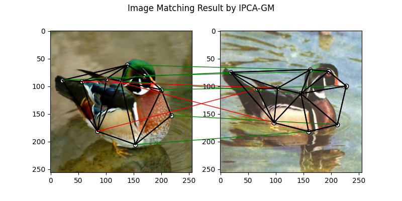
Matching by IPCA-GM model
See ipca_gm() for the API reference.
path = pygm.utils.download('vgg16_ipca_voc_jittor.pt', 'https://drive.google.com/u/0/uc?export=download&confirm=Z-AR&id=1f7KEl9ZFZwI26j6UId-fsdl8Y8QWPKZi')
cnn.load_state_dict(jt.load(path))

feat1_local, feat1_global = cnn(jittor_img1)
feat2_local, feat2_global = cnn(jittor_img2)
Normalize the features
def l2norm(node_feat):
    return local_response_norm(
        node_feat, node_feat.shape[1] * 2, alpha=node_feat.shape[1] * 2, beta=0.5, k=0)

feat1_local = l2norm(feat1_local)
feat1_global = l2norm(feat1_global)
feat2_local = l2norm(feat2_local)
feat2_global = l2norm(feat2_global)
Up-sample the features to the original image size and concatenate
feat1_local_upsample = jt.nn.interpolate(feat1_local, (obj_resize[1], obj_resize[0]), mode='bilinear')
feat1_global_upsample = jt.nn.interpolate(feat1_global, (obj_resize[1], obj_resize[0]), mode='bilinear')
feat2_local_upsample = jt.nn.interpolate(feat2_local, (obj_resize[1], obj_resize[0]), mode='bilinear')
feat2_global_upsample = jt.nn.interpolate(feat2_global, (obj_resize[1], obj_resize[0]), mode='bilinear')
feat1_upsample = jt.concat((feat1_local_upsample, feat1_global_upsample), dim=1)
feat2_upsample = jt.concat((feat2_local_upsample, feat2_global_upsample), dim=1)
num_features = feat1_upsample.shape[1]
Extract node features by nearest interpolation
rounded_kpts1 = jt.round(kpts1).long()
rounded_kpts2 = jt.round(kpts2).long()
node1 = feat1_upsample[0, :, rounded_kpts1[1], rounded_kpts1[0]].t() # shape: NxC
node2 = feat2_upsample[0, :, rounded_kpts2[1], rounded_kpts2[0]].t() # shape: NxC
Build edge features as edge lengths
kpts1_dis = (kpts1.unsqueeze(0) - kpts1.unsqueeze(1))
kpts1_dis = jt.norm(kpts1_dis, p=2, dim=2).detach()
kpts2_dis = (kpts2.unsqueeze(0) - kpts2.unsqueeze(1))
kpts2_dis = jt.norm(kpts2_dis, p=2, dim=2).detach()

Q1 = jt.exp(-kpts1_dis / obj_resize[0])
Q2 = jt.exp(-kpts2_dis / obj_resize[0])
Matching by IPCA-GM model
X = pygm.ipca_gm(node1, node2, A1, A2, pretrain='voc')
X = pygm.hungarian(X)

plt.figure(figsize=(8, 4))
plt.suptitle('Image Matching Result by IPCA-GM')
ax1 = plt.subplot(1, 2, 1)
plot_image_with_graph(img1, kpts1, A1)
ax2 = plt.subplot(1, 2, 2)
plot_image_with_graph(img2, kpts2, A2)
idx, _ = jt.argmax(X, dim=1)
for i in range(X.shape[0]):
    j = idx[i].item()
    con = ConnectionPatch(xyA=kpts1[:, i], xyB=kpts2[:, j], coordsA="data", coordsB="data",
                          axesA=ax1, axesB=ax2, color="red" if i != j else "green")
    plt.gca().add_artist(con)
Matching by CIE model
See cie() for the API reference.
path = pygm.utils.download('vgg16_cie_voc_jittor.pt', 'https://drive.google.com/u/0/uc?export=download&confirm=Z-AR&id=1wDbA-8sK4BNhA48z2c-Gtdd4AarRxfqT')
cnn.load_state_dict(jt.load(path))

feat1_local, feat1_global = cnn(jittor_img1)
feat2_local, feat2_global = cnn(jittor_img2)
Normalize the features
def l2norm(node_feat):
    return local_response_norm(
        node_feat, node_feat.shape[1] * 2, alpha=node_feat.shape[1] * 2, beta=0.5, k=0)

feat1_local = l2norm(feat1_local)
feat1_global = l2norm(feat1_global)
feat2_local = l2norm(feat2_local)
feat2_global = l2norm(feat2_global)
Up-sample the features to the original image size and concatenate
feat1_local_upsample = jt.nn.interpolate(feat1_local, (obj_resize[1], obj_resize[0]), mode='bilinear')
feat1_global_upsample = jt.nn.interpolate(feat1_global, (obj_resize[1], obj_resize[0]), mode='bilinear')
feat2_local_upsample = jt.nn.interpolate(feat2_local, (obj_resize[1], obj_resize[0]), mode='bilinear')
feat2_global_upsample = jt.nn.interpolate(feat2_global, (obj_resize[1], obj_resize[0]), mode='bilinear')
feat1_upsample = jt.concat((feat1_local_upsample, feat1_global_upsample), dim=1)
feat2_upsample = jt.concat((feat2_local_upsample, feat2_global_upsample), dim=1)
num_features = feat1_upsample.shape[1]
Extract node features by nearest interpolation
rounded_kpts1 = jt.round(kpts1).long()
rounded_kpts2 = jt.round(kpts2).long()
node1 = feat1_upsample[0, :, rounded_kpts1[1], rounded_kpts1[0]].t() # shape: NxC
node2 = feat2_upsample[0, :, rounded_kpts2[1], rounded_kpts2[0]].t() # shape: NxC
Build edge features as edge lengths
kpts1_dis = (kpts1.unsqueeze(1) - kpts1.unsqueeze(2))
kpts1_dis = jt.norm(kpts1_dis, p=2, dim=0).detach()
kpts2_dis = (kpts2.unsqueeze(1) - kpts2.unsqueeze(2))
kpts2_dis = jt.norm(kpts2_dis, p=2, dim=0).detach()

Q1 = jt.exp(-kpts1_dis / obj_resize[0]).unsqueeze(-1).float32()
Q2 = jt.exp(-kpts2_dis / obj_resize[0]).unsqueeze(-1).float32()
Call CIE matching model
X = pygm.cie(node1, node2, A1, A2, Q1, Q2, pretrain='voc')
X = pygm.hungarian(X)

plt.figure(figsize=(8, 4))
plt.suptitle('Image Matching Result by CIE')
ax1 = plt.subplot(1, 2, 1)
plot_image_with_graph(img1, kpts1, A1)
ax2 = plt.subplot(1, 2, 2)
plot_image_with_graph(img2, kpts2, A2)
idx, _ = jt.argmax(X, dim=1)
for i in range(X.shape[0]):
    j = idx[i].item()
    con = ConnectionPatch(xyA=kpts1[:, i], xyB=kpts2[:, j], coordsA="data", coordsB="data",
                          axesA=ax1, axesB=ax2, color="red" if i != j else "green")
    plt.gca().add_artist(con)

Training a deep graph matching model
In this section, we show how to build a deep graph matching model which supports end-to-end training. For the image matching problem considered here, the model is composed of a CNN feature extractor and a learnable matching module. Take the PCA-GM model as an example.
Note
This simple example is intended to show you how to do the basic execute and backward pass when training an end-to-end deep graph matching neural network. A ‘more formal’ deep learning pipeline should involve asynchronized data loader, batched operations, CUDA support and so on, which are all omitted in consideration of simplicity. You may refer to ThinkMatch which is a research protocol with all these advanced features.
Let’s firstly define the neural network model. By calling get_network(),
it will simply return the network object.
class GMNet(jt.nn.Module):
    def __init__(self):
        super(GMNet, self).__init__()
        self.gm_net = pygm.utils.get_network(pygm.pca_gm, pretrain=False) # fetch the network object
        self.cnn = CNNNet(vgg16_cnn)

    def execute(self, img1, img2, kpts1, kpts2, A1, A2):
        # CNN feature extractor layers
        feat1_local, feat1_global = self.cnn(img1)
        feat2_local, feat2_global = self.cnn(img2)
        feat1_local = l2norm(feat1_local)
        feat1_global = l2norm(feat1_global)
        feat2_local = l2norm(feat2_local)
        feat2_global = l2norm(feat2_global)

        # upsample feature map
        feat1_local_upsample = jt.nn.interpolate(feat1_local, (obj_resize[1], obj_resize[0]), mode='bilinear')
        feat1_global_upsample = jt.nn.interpolate(feat1_global, (obj_resize[1], obj_resize[0]), mode='bilinear')
        feat2_local_upsample = jt.nn.interpolate(feat2_local, (obj_resize[1], obj_resize[0]), mode='bilinear')
        feat2_global_upsample = jt.nn.interpolate(feat2_global, (obj_resize[1], obj_resize[0]), mode='bilinear')
        feat1_upsample = jt.concat((feat1_local_upsample, feat1_global_upsample), dim=1)
        feat2_upsample = jt.concat((feat2_local_upsample, feat2_global_upsample), dim=1)

        # assign node features
        rounded_kpts1 = jt.round(kpts1).long()
        rounded_kpts2 = jt.round(kpts2).long()
        node1 = feat1_upsample[0, :, rounded_kpts1[1], rounded_kpts1[0]].t()  # shape: NxC
        node2 = feat2_upsample[0, :, rounded_kpts2[1], rounded_kpts2[0]].t()  # shape: NxC

        # PCA-GM matching layers
        X = pygm.pca_gm(node1, node2, A1, A2, network=self.gm_net) # the network object is reused
        return X

model = GMNet()
Define optimizer
optim = jt.optim.Adam(model.parameters(), lr=1e-3)
Forward pass
X = model(jittor_img1, jittor_img2, kpts1, kpts2, A1, A2)
Compute loss
In this example, the ground truth matching matrix is a diagonal matrix. We calculate the loss function via
permutation_loss()
X_gt = jt.init.eye(X.shape[0])
loss = pygm.utils.permutation_loss(X, X_gt)
print(f'loss={loss:.4f}')
loss=2.9790
Backward Pass
optim.backward(loss)
Visualize the gradients
plt.figure(figsize=(4, 4))
plt.title('Gradient Sizes of PCA-GM and VGG16 layers')
plt.gca().set_xlabel('Layer Index')
plt.gca().set_ylabel('Average Gradient Size')
grad_size = []
for param in model.parameters():
    grad_size.append(jt.abs(param.opt_grad(optim)).mean().item())
print(grad_size)
plt.stem(grad_size)
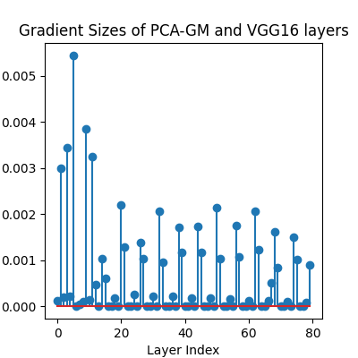
[0.00012032000813633204, 0.0029908756259828806, 0.0001890812418423593, 0.003432080615311861, 0.0002175412664655596, 0.005439706612378359, 8.84531982592307e-06, 4.3844393076142296e-05, 9.275232150685042e-05, 0.0038394334260374308, 0.00014068347809370607, 0.0032387105748057365, 0.0004730010114144534, 2.232744122920849e-08, 0.0010210294276475906, 0.0005979313282296062, 0.0, 0.0, 0.0001719535794109106, 1.1543310307615684e-08, 0.0021903959568589926, 0.0012790058972314, 0.0, 0.0, 0.00025605762493796647, 3.661839054203142e-09, 0.0013879203470423818, 0.001030159299261868, 0.0, 0.0, 0.0002153523819288239, 4.659028274289767e-09, 0.0020632531959563494, 0.0009495018748566508, 0.0, 0.0, 0.00020805593521799892, 1.3135081911030966e-09, 0.0017076103249564767, 0.0011711850529536605, 0.0, 0.0, 0.00017217609274666756, 2.7571318561570024e-09, 0.001730420277453959, 0.0011667078360915184, 0.0, 0.0, 0.00018079271831084043, 3.229687406403059e-09, 0.0021298921201378107, 0.001029890263453126, 0.0, 0.0, 0.0001582755212439224, 7.906685861591711e-10, 0.0017488845624029636, 0.0010780903976410627, 0.0, 0.0, 0.0001245360035682097, 1.4797246761233396e-09, 0.00206647627055645, 0.0012257269117981195, 0.0, 0.0, 0.00012214107846375555, 0.0005140944267623127, 0.001602952484972775, 0.0008278230670839548, 0.0, 0.0, 9.437291737413034e-05, 4.0557557312581594e-10, 0.0014863943215459585, 0.0010152073809877038, 0.0, 0.0, 8.532514766557142e-05, 0.000895310309715569]

<StemContainer object of 3 artists>
Update the model parameters. A deep learning pipeline should iterate the forward pass and backward pass steps until convergence.
optim.step()
optim.zero_grad()
Note
This example supports both GPU and CPU, and the online documentation is built by a CPU-only machine. The efficiency will be significantly improved if you run this code on GPU.
Total running time of the script: (1 minutes 12.772 seconds)