Discovering Subgraphs

This example shows how to match a smaller graph to a subset of a larger graph.

# Author: Runzhong Wang <runzhong.wang@sjtu.edu.cn>
#         Qi Liu <purewhite@sjtu.edu.cn>
#
# License: Mulan PSL v2 License

Note

The following solvers are included in this example:

• rrwm() (classic solver)

• ipfp() (classic solver)

• sm() (classic solver)

• ngm() (neural network solver)

import jittor as jt # jittor backend
import pygmtools as pygm
import matplotlib.pyplot as plt # for plotting
from matplotlib.patches import ConnectionPatch # for plotting matching result
import networkx as nx # for plotting graphs
pygm.BACKEND = 'jittor' # set default backend for pygmtools
_ = jt.set_seed(1) # fix random seed

# jt.flags.use_cuda = 1 # use cuda

#! The following code is used for testing jittor codes.
import numpy as np

def namestr(obj):
 return [name for name in globals() if globals()[name] is obj][0]

def load_var(*args):
    ret = []
    for var in args:
        ret.append(jt.Var(np.load(f'../{namestr(var)}.npy')))
    return ret


def compare_var(*args):
    for var in args:
        var_np = np.load(f'../{namestr(var)}.npy')
        assert np.allclose(var.numpy(), var_np, rtol=1e-4)

Generate the larger graph

num_nodes2 = 10
A2 = jt.rand(num_nodes2, num_nodes2)
A2 = (A2 + A2.t() > 1.) * (A2 + A2.t()) / 2
A2[jt.arange(A2.shape[0]), jt.arange(A2.shape[0])] = 0
n2 = jt.Var([num_nodes2])

Generate the smaller graph

num_nodes1 = 5
G2 = nx.from_numpy_array(A2.numpy())
pos2 = nx.spring_layout(G2)
pos2_t = jt.Var([pos2[_] for _ in range(num_nodes2)])
selected = [0] # build G1 as a cluster in visualization
unselected = list(range(1, num_nodes2))
while len(selected) < num_nodes1:
    dist = jt.sum(jt.sum(jt.abs(pos2_t[selected].unsqueeze(1) - pos2_t[unselected].unsqueeze(0)), dim=-1), dim=0)
    select_id = unselected[jt.argmin(dist, dim=-1)[0].item()] # find the closest node from unselected
    selected.append(select_id)
    unselected.remove(select_id)
selected.sort()
A1 = A2[selected, :][:, selected]
X_gt = jt.init.eye(num_nodes2)[selected, :]
n1 = jt.Var([num_nodes1])

Visualize the graphs

G1 = nx.from_numpy_array(A1.numpy())
pos1 = {_: pos2[selected[_]] for _ in range(num_nodes1)}
color1 = ['#FF5733' for _ in range(num_nodes1)]
color2 = ['#FF5733' if _ in selected else '#1f78b4' for _ in range(num_nodes2)]
plt.figure(figsize=(8, 4))
plt.subplot(1, 2, 1)
plt.title('Subgraph 1')
plt.gca().margins(0.4)
nx.draw_networkx(G1, pos=pos1, node_color=color1)
plt.subplot(1, 2, 2)
plt.title('Graph 2')
nx.draw_networkx(G2, pos=pos2, node_color=color2)

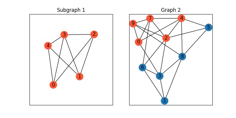
We then show how to automatically discover the matching by graph matching.

Build affinity matrix

To match the larger graph and the smaller graph, we follow the formulation of Quadratic Assignment Problem (QAP):

\[\begin{split}&\max_{\mathbf{X}} \ \texttt{vec}(\mathbf{X})^\top \mathbf{K} \texttt{vec}(\mathbf{X})\\ s.t. \quad &\mathbf{X} \in \{0, 1\}^{n_1\times n_2}, \ \mathbf{X}\mathbf{1} = \mathbf{1}, \ \mathbf{X}^\top\mathbf{1} \leq \mathbf{1}\end{split}\]

where the first step is to build the affinity matrix (\(\mathbf{K}\))

conn1, edge1 = pygm.utils.dense_to_sparse(A1)
conn2, edge2 = pygm.utils.dense_to_sparse(A2)
import functools
gaussian_aff = functools.partial(pygm.utils.gaussian_aff_fn, sigma=.001) # set affinity function
K = pygm.utils.build_aff_mat(None, edge1, conn1, None, edge2, conn2, n1, None, n2, None, edge_aff_fn=gaussian_aff)

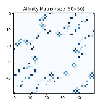
Visualization of the affinity matrix. For graph matching problem with \(N_1\) and \(N_2\) nodes, the affinity matrix has \(N_1N_2\times N_1N_2\) elements because there are \(N_1^2\) and \(N_2^2\) edges in each graph, respectively.

Note

The diagonal elements of the affinity matrix is empty because there is no node features in this example.

plt.figure(figsize=(4, 4))
plt.title(f'Affinity Matrix (size: {K.shape[0]}$\\times${K.shape[1]})')
plt.imshow(K.numpy(), cmap='Blues')

<matplotlib.image.AxesImage object at 0x000001F03D1EAFD0>

Solve graph matching problem by RRWM solver

See rrwm() for the API reference.

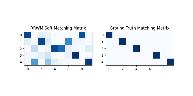
X = pygm.rrwm(K, n1, n2)

The output of RRWM is a soft matching matrix. Visualization:

plt.figure(figsize=(8, 4))
plt.subplot(1, 2, 1)
plt.title('RRWM Soft Matching Matrix')
plt.imshow(X.numpy(), cmap='Blues')
plt.subplot(1, 2, 2)
plt.title('Ground Truth Matching Matrix')
plt.imshow(X_gt.numpy(), cmap='Blues')

<matplotlib.image.AxesImage object at 0x000001F03DE77D60>

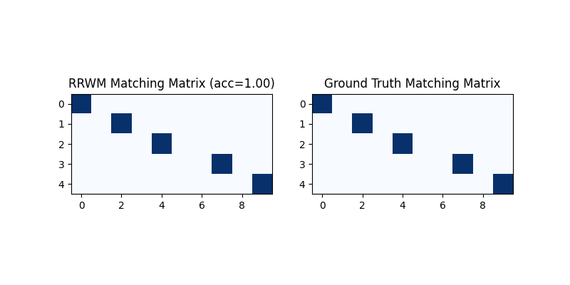
Get the discrete matching matrix

Hungarian algorithm is then adopted to reach a discrete matching matrix

X = pygm.hungarian(X)

Visualization of the discrete matching matrix:

plt.figure(figsize=(8, 4))
plt.subplot(1, 2, 1)
plt.title(f'RRWM Matching Matrix (acc={(X * X_gt).sum()/ X_gt.sum():.2f})')
plt.imshow(X.numpy(), cmap='Blues')
plt.subplot(1, 2, 2)
plt.title('Ground Truth Matching Matrix')
plt.imshow(X_gt.numpy(), cmap='Blues')

<matplotlib.image.AxesImage object at 0x000001F03E467970>

Match the subgraph

Draw the matching:

plt.figure(figsize=(8, 4))
plt.suptitle(f'RRWM Matching Result (acc={(X * X_gt).sum()/ X_gt.sum():.2f})')
ax1 = plt.subplot(1, 2, 1)
plt.title('Subgraph 1')
plt.gca().margins(0.4)
nx.draw_networkx(G1, pos=pos1, node_color=color1)
ax2 = plt.subplot(1, 2, 2)
plt.title('Graph 2')
nx.draw_networkx(G2, pos=pos2, node_color=color2)
for i in range(num_nodes1):
    j = jt.argmax(X[i], dim=-1)[0].item()
    con = ConnectionPatch(xyA=pos1[i], xyB=pos2[j], coordsA="data", coordsB="data",
                          axesA=ax1, axesB=ax2, color="green" if X_gt[i,j] == 1 else "red")
    plt.gca().add_artist(con)

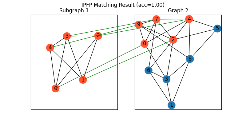
Other solvers are also available

Classic IPFP solver

See ipfp() for the API reference.

X = pygm.ipfp(K, n1, n2)

Visualization of IPFP matching result:

plt.figure(figsize=(8, 4))
plt.suptitle(f'IPFP Matching Result (acc={(X * X_gt).sum()/ X_gt.sum():.2f})')
ax1 = plt.subplot(1, 2, 1)
plt.title('Subgraph 1')
plt.gca().margins(0.4)
nx.draw_networkx(G1, pos=pos1, node_color=color1)
ax2 = plt.subplot(1, 2, 2)
plt.title('Graph 2')
nx.draw_networkx(G2, pos=pos2, node_color=color2)
for i in range(num_nodes1):
    j = jt.argmax(X[i], dim=-1)[0].item()
    con = ConnectionPatch(xyA=pos1[i], xyB=pos2[j], coordsA="data", coordsB="data",
                          axesA=ax1, axesB=ax2, color="green" if X_gt[i,j] == 1 else "red")
    plt.gca().add_artist(con)

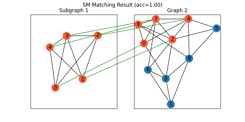
Classic SM solver

See sm() for the API reference.

X = pygm.sm(K, n1, n2)
X = pygm.hungarian(X)

Visualization of SM matching result:

plt.figure(figsize=(8, 4))
plt.suptitle(f'SM Matching Result (acc={(X * X_gt).sum()/ X_gt.sum():.2f})')
ax1 = plt.subplot(1, 2, 1)
plt.title('Subgraph 1')
plt.gca().margins(0.4)
nx.draw_networkx(G1, pos=pos1, node_color=color1)
ax2 = plt.subplot(1, 2, 2)
plt.title('Graph 2')
nx.draw_networkx(G2, pos=pos2, node_color=color2)
for i in range(num_nodes1):
    j = jt.argmax(X[i], dim=-1)[0].item()
    con = ConnectionPatch(xyA=pos1[i], xyB=pos2[j], coordsA="data", coordsB="data",
                          axesA=ax1, axesB=ax2, color="green" if X_gt[i,j] == 1 else "red")
    plt.gca().add_artist(con)

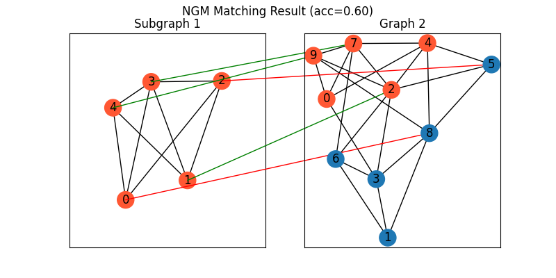
NGM neural network solver

See ngm() for the API reference.

Note

The NGM solvers are pretrained on a different problem setting, so their performance may seem inferior. To improve their performance, you may change the way of building affinity matrices, or try finetuning NGM on the new problem.

with jt.no_grad():
    X = pygm.ngm(K, n1, n2, pretrain='voc')
    X = pygm.hungarian(X)

Visualization of NGM matching result:

plt.figure(figsize=(8, 4))
plt.suptitle(f'NGM Matching Result (acc={(X * X_gt).sum()/ X_gt.sum():.2f})')
ax1 = plt.subplot(1, 2, 1)
plt.title('Subgraph 1')
plt.gca().margins(0.4)
nx.draw_networkx(G1, pos=pos1, node_color=color1)
ax2 = plt.subplot(1, 2, 2)
plt.title('Graph 2')
nx.draw_networkx(G2, pos=pos2, node_color=color2)
for i in range(num_nodes1):
    j = jt.argmax(X[i], dim=-1)[0].item()
    con = ConnectionPatch(xyA=pos1[i], xyB=pos2[j], coordsA="data", coordsB="data",
                          axesA=ax1, axesB=ax2, color="green" if X_gt[i,j] == 1 else "red")
    plt.gca().add_artist(con)