Introduction: Matching Isomorphic Graphs

This example is an introduction to pygmtools which shows how to match isomorphic graphs. Isomorphic graphs means graphs whose structures are identical, but the node correspondence is unknown.

# Author: Runzhong Wang <runzhong.wang@sjtu.edu.cn>
#
# License: Mulan PSL v2 License

Note

The following solvers support QAP formulation, and are included in this example:

• rrwm() (classic solver)

• ipfp() (classic solver)

• sm() (classic solver)

• ngm() (neural network solver)

import torch # pytorch backend
import pygmtools as pygm
import matplotlib.pyplot as plt # for plotting
from matplotlib.patches import ConnectionPatch # for plotting matching result
import networkx as nx # for plotting graphs
pygm.BACKEND = 'pytorch' # set default backend for pygmtools
_ = torch.manual_seed(1) # fix random seed

Generate two isomorphic graphs

num_nodes = 10
X_gt = torch.zeros(num_nodes, num_nodes)
X_gt[torch.arange(0, num_nodes, dtype=torch.int64), torch.randperm(num_nodes)] = 1
A1 = torch.rand(num_nodes, num_nodes)
A1 = (A1 + A1.t() > 1.) * (A1 + A1.t()) / 2
torch.diagonal(A1)[:] = 0
A2 = torch.mm(torch.mm(X_gt.t(), A1), X_gt)
n1 = torch.tensor([num_nodes])
n2 = torch.tensor([num_nodes])

Visualize the graphs

plt.figure(figsize=(8, 4))
G1 = nx.from_numpy_array(A1.numpy())
G2 = nx.from_numpy_array(A2.numpy())
pos1 = nx.spring_layout(G1)
pos2 = nx.spring_layout(G2)
plt.subplot(1, 2, 1)
plt.title('Graph 1')
nx.draw_networkx(G1, pos=pos1)
plt.subplot(1, 2, 2)
plt.title('Graph 2')
nx.draw_networkx(G2, pos=pos2)

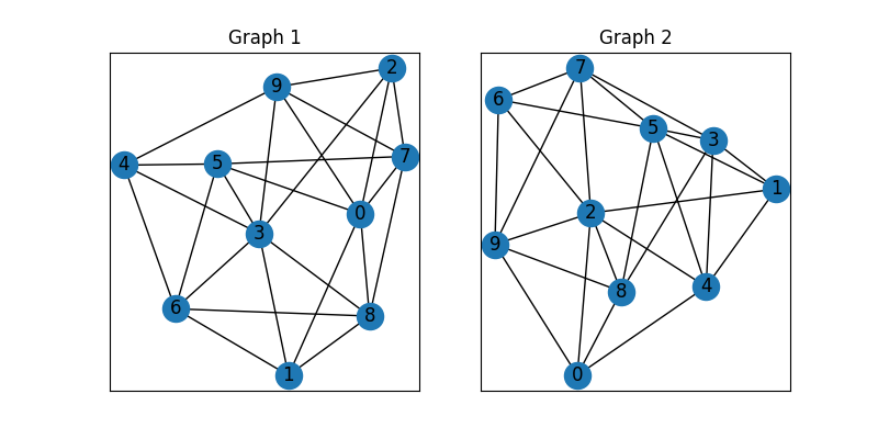
These two graphs look dissimilar because they are not aligned. We then align these two graphs by graph matching.

Build affinity matrix

To match isomorphic graphs by graph matching, we follow the formulation of Quadratic Assignment Problem (QAP):

\[\begin{split}&\max_{\mathbf{X}} \ \texttt{vec}(\mathbf{X})^\top \mathbf{K} \texttt{vec}(\mathbf{X})\\ s.t. \quad &\mathbf{X} \in \{0, 1\}^{n_1\times n_2}, \ \mathbf{X}\mathbf{1} = \mathbf{1}, \ \mathbf{X}^\top\mathbf{1} \leq \mathbf{1}\end{split}\]

where the first step is to build the affinity matrix (\(\mathbf{K}\))

conn1, edge1 = pygm.utils.dense_to_sparse(A1)
conn2, edge2 = pygm.utils.dense_to_sparse(A2)
import functools
gaussian_aff = functools.partial(pygm.utils.gaussian_aff_fn, sigma=.1) # set affinity function
K = pygm.utils.build_aff_mat(None, edge1, conn1, None, edge2, conn2, n1, None, n2, None, edge_aff_fn=gaussian_aff)

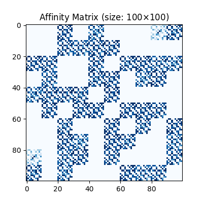
Visualization of the affinity matrix. For graph matching problem with \(N\) nodes, the affinity matrix has \(N^2\times N^2\) elements because there are \(N^2\) edges in each graph.

Note

The diagonal elements of the affinity matrix is empty because there is no node features in this example.

plt.figure(figsize=(4, 4))
plt.title(f'Affinity Matrix (size: {K.shape[0]}$\\times${K.shape[1]})')
plt.imshow(K.numpy(), cmap='Blues')

<matplotlib.image.AxesImage object at 0x00000221B6EDC850>

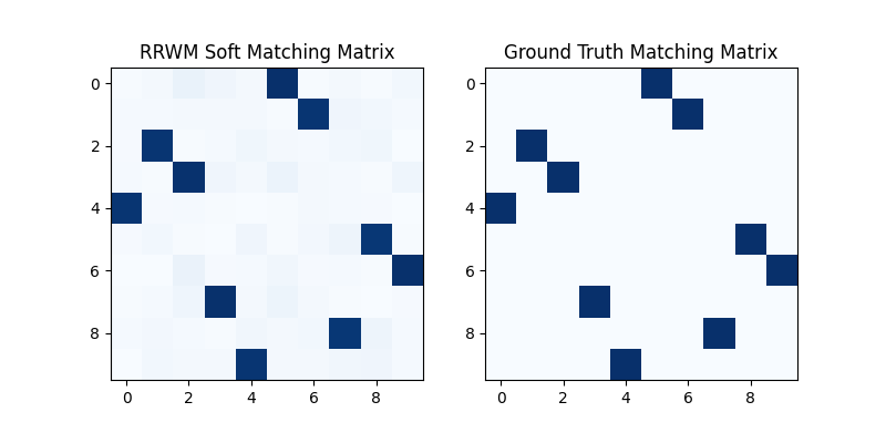
Solve graph matching problem by RRWM solver

See rrwm() for the API reference.

X = pygm.rrwm(K, n1, n2)

The output of RRWM is a soft matching matrix. Visualization:

plt.figure(figsize=(8, 4))
plt.subplot(1, 2, 1)
plt.title('RRWM Soft Matching Matrix')
plt.imshow(X.numpy(), cmap='Blues')
plt.subplot(1, 2, 2)
plt.title('Ground Truth Matching Matrix')
plt.imshow(X_gt.numpy(), cmap='Blues')

<matplotlib.image.AxesImage object at 0x00000221B7671910>

Get the discrete matching matrix

Hungarian algorithm is then adopted to reach a discrete matching matrix

X = pygm.hungarian(X)

Visualization of the discrete matching matrix:

plt.figure(figsize=(8, 4))
plt.subplot(1, 2, 1)
plt.title(f'RRWM Matching Matrix (acc={(X * X_gt).sum()/ X_gt.sum():.2f})')
plt.imshow(X.numpy(), cmap='Blues')
plt.subplot(1, 2, 2)
plt.title('Ground Truth Matching Matrix')
plt.imshow(X_gt.numpy(), cmap='Blues')

<matplotlib.image.AxesImage object at 0x00000221B785ED60>

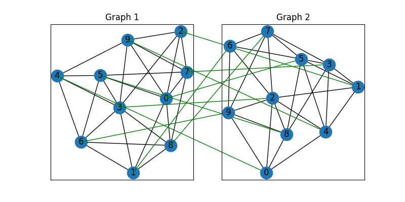
Align the original graphs

Draw the matching (green lines for correct matching, red lines for wrong matching):

plt.figure(figsize=(8, 4))
ax1 = plt.subplot(1, 2, 1)
plt.title('Graph 1')
nx.draw_networkx(G1, pos=pos1)
ax2 = plt.subplot(1, 2, 2)
plt.title('Graph 2')
nx.draw_networkx(G2, pos=pos2)
for i in range(num_nodes):
    j = torch.argmax(X[i]).item()
    con = ConnectionPatch(xyA=pos1[i], xyB=pos2[j], coordsA="data", coordsB="data",
                          axesA=ax1, axesB=ax2, color="green" if X_gt[i, j] else "red")
    plt.gca().add_artist(con)

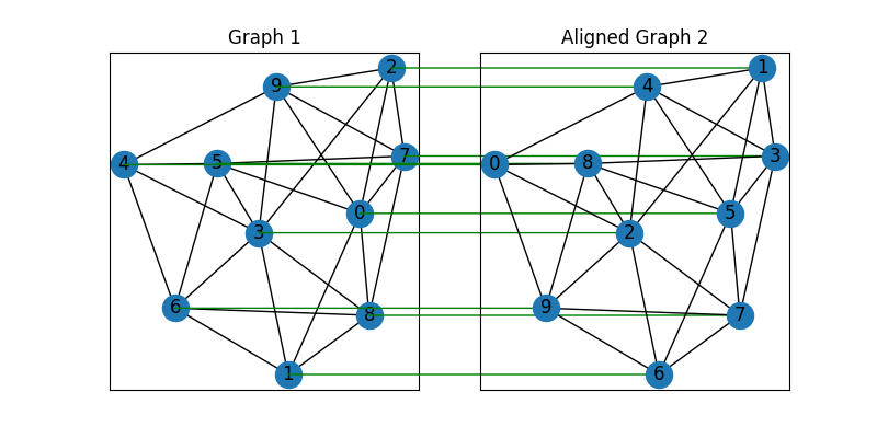
Align the nodes:

align_A2 = torch.mm(torch.mm(X, A2), X.t())
plt.figure(figsize=(8, 4))
ax1 = plt.subplot(1, 2, 1)
plt.title('Graph 1')
nx.draw_networkx(G1, pos=pos1)
ax2 = plt.subplot(1, 2, 2)
plt.title('Aligned Graph 2')
align_pos2 = {}
for i in range(num_nodes):
    j = torch.argmax(X[i]).item()
    align_pos2[j] = pos1[i]
    con = ConnectionPatch(xyA=pos1[i], xyB=align_pos2[j], coordsA="data", coordsB="data",
                          axesA=ax1, axesB=ax2, color="green" if X_gt[i, j] else "red")
    plt.gca().add_artist(con)
nx.draw_networkx(G2, pos=align_pos2)

Other solvers are also available

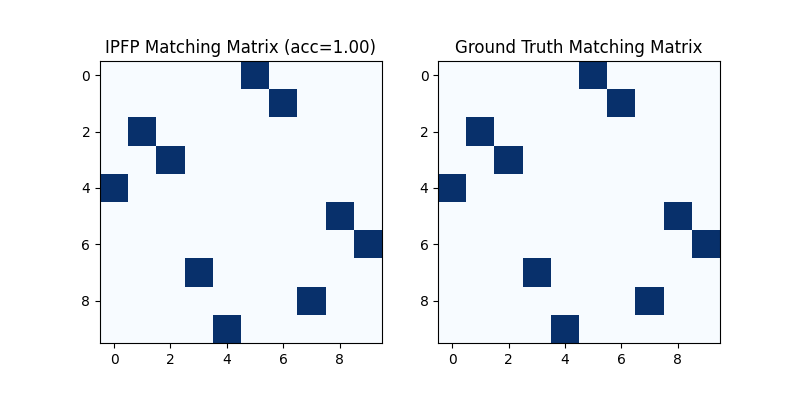
Classic IPFP solver

See ipfp() for the API reference.

X = pygm.ipfp(K, n1, n2)

Visualization of IPFP matching result:

plt.figure(figsize=(8, 4))
plt.subplot(1, 2, 1)
plt.title(f'IPFP Matching Matrix (acc={(X * X_gt).sum()/ X_gt.sum():.2f})')
plt.imshow(X.numpy(), cmap='Blues')
plt.subplot(1, 2, 2)
plt.title('Ground Truth Matching Matrix')
plt.imshow(X_gt.numpy(), cmap='Blues')

<matplotlib.image.AxesImage object at 0x00000221B6597160>

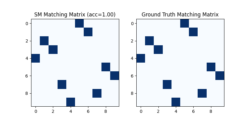
Classic SM solver

See sm() for the API reference.

X = pygm.sm(K, n1, n2)
X = pygm.hungarian(X)

Visualization of SM matching result:

plt.figure(figsize=(8, 4))
plt.subplot(1, 2, 1)
plt.title(f'SM Matching Matrix (acc={(X * X_gt).sum()/ X_gt.sum():.2f})')
plt.imshow(X.numpy(), cmap='Blues')
plt.subplot(1, 2, 2)
plt.title('Ground Truth Matching Matrix')
plt.imshow(X_gt.numpy(), cmap='Blues')

<matplotlib.image.AxesImage object at 0x00000221B663ED90>

NGM neural network solver

See ngm() for the API reference.

with torch.set_grad_enabled(False):
    X = pygm.ngm(K, n1, n2, pretrain='voc')
    X = pygm.hungarian(X)

Visualization of NGM matching result:

plt.figure(figsize=(8, 4))
plt.subplot(1, 2, 1)
plt.title(f'NGM Matching Matrix (acc={(X * X_gt).sum()/ X_gt.sum():.2f})')
plt.imshow(X.numpy(), cmap='Blues')
plt.subplot(1, 2, 2)
plt.title('Ground Truth Matching Matrix')
plt.imshow(X_gt.numpy(), cmap='Blues')

<matplotlib.image.AxesImage object at 0x00000221B7E39C70>