Seeded Graph Matching

Seeded graph matching means some partial of the matching result is already known, and the known matching results are called “seeds”. In this example, we show how to exploit such prior with pygmtools.

# Author: Runzhong Wang <runzhong.wang@sjtu.edu.cn>
#
# License: Mulan PSL v2 License

Note

How to perform seeded graph matching is still an open research problem. In this example, we show a simple yet effective approach that works with pygmtools.

Note

The following solvers are included in this example:

• rrwm() (classic solver)

• ipfp() (classic solver)

• sm() (classic solver)

• ngm() (neural network solver)

import torch # pytorch backend
import pygmtools as pygm
import matplotlib.pyplot as plt # for plotting
from matplotlib.patches import ConnectionPatch # for plotting matching result
import networkx as nx # for plotting graphs
pygm.BACKEND = 'pytorch' # set default backend for pygmtools
_ = torch.manual_seed(1) # fix random seed

Generate two isomorphic graphs (with seeds)

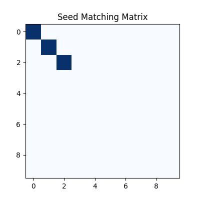
In this example, we assume the first three nodes are already aligned. Firstly, we generate the seed matching matrix:

num_nodes = 10
num_seeds = 3
seed_mat = torch.zeros(num_nodes, num_nodes)
seed_mat[:num_seeds, :num_seeds] = torch.eye(num_seeds)

Then we generate the isomorphic graphs:

X_gt = seed_mat.clone()
X_gt[num_seeds:, num_seeds:][torch.arange(0, num_nodes-num_seeds, dtype=torch.int64), torch.randperm(num_nodes-num_seeds)] = 1
A1 = torch.rand(num_nodes, num_nodes)
A1 = (A1 + A1.t() > 1.) * (A1 + A1.t()) / 2
torch.diagonal(A1)[:] = 0
A2 = torch.mm(torch.mm(X_gt.t(), A1), X_gt)
n1 = torch.tensor([num_nodes])
n2 = torch.tensor([num_nodes])

Visualize the graphs and seeds

The seed matching matrix:

plt.figure(figsize=(4, 4))
plt.title('Seed Matching Matrix')
plt.imshow(seed_mat.numpy(), cmap='Blues')

<matplotlib.image.AxesImage object at 0x00000221B7FC1F70>

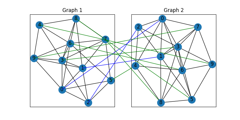
The blue lines denote the matching seeds.

plt.figure(figsize=(8, 4))
G1 = nx.from_numpy_array(A1.numpy())
G2 = nx.from_numpy_array(A2.numpy())
pos1 = nx.spring_layout(G1)
pos2 = nx.spring_layout(G2)
ax1 = plt.subplot(1, 2, 1)
plt.title('Graph 1')
nx.draw_networkx(G1, pos=pos1)
ax2 = plt.subplot(1, 2, 2)
plt.title('Graph 2')
nx.draw_networkx(G2, pos=pos2)
for i in range(num_seeds):
    j = torch.argmax(seed_mat[i]).item()
    con = ConnectionPatch(xyA=pos1[i], xyB=pos2[j], coordsA="data", coordsB="data",
                          axesA=ax1, axesB=ax2, color="blue")
    plt.gca().add_artist(con)

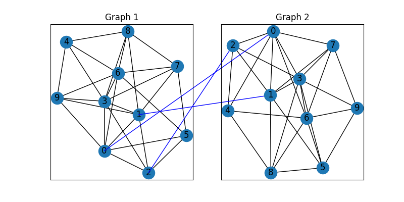
Now these two graphs look dissimilar because they are not aligned. We then align these two graphs by graph matching.

Build affinity matrix with seed prior

We follow the formulation of Quadratic Assignment Problem (QAP):

\[\begin{split}&\max_{\mathbf{X}} \ \texttt{vec}(\mathbf{X})^\top \mathbf{K} \texttt{vec}(\mathbf{X})\\ s.t. \quad &\mathbf{X} \in \{0, 1\}^{n_1\times n_2}, \ \mathbf{X}\mathbf{1} = \mathbf{1}, \ \mathbf{X}^\top\mathbf{1} \leq \mathbf{1}\end{split}\]

where the first step is to build the affinity matrix (\(\mathbf{K}\)). We firstly build a “standard” affinity matrix:

conn1, edge1 = pygm.utils.dense_to_sparse(A1)
conn2, edge2 = pygm.utils.dense_to_sparse(A2)
import functools
gaussian_aff = functools.partial(pygm.utils.gaussian_aff_fn, sigma=.1) # set affinity function
K = pygm.utils.build_aff_mat(None, edge1, conn1, None, edge2, conn2, n1, None, n2, None, edge_aff_fn=gaussian_aff)

The next step is to add the seed matching information as priors to the affinity matrix. The matching priors are treated as node affinities and the corresponding node affinity is added by 10 if there is an matching prior.

Note

The node affinity matrix is transposed because in the graph matching formulation followed by pygmtools, \(\texttt{vec}(\mathbf{X})\) means column vectorization. The node affinity should also be column- vectorized.

torch.diagonal(K)[:] += seed_mat.t().reshape(-1) * 10

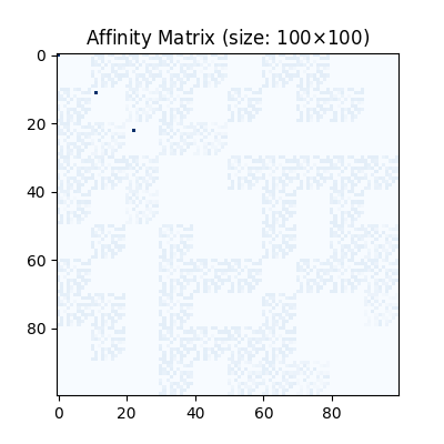
Visualization of the affinity matrix.

Note

In this example, the diagonal elements reflect the matching prior.

plt.figure(figsize=(4, 4))
plt.title(f'Affinity Matrix (size: {K.shape[0]}$\\times${K.shape[1]})')
plt.imshow(K.numpy(), cmap='Blues')

<matplotlib.image.AxesImage object at 0x00000221B7653940>

Solve graph matching problem by RRWM solver

See rrwm() for the API reference.

X = pygm.rrwm(K, n1, n2)

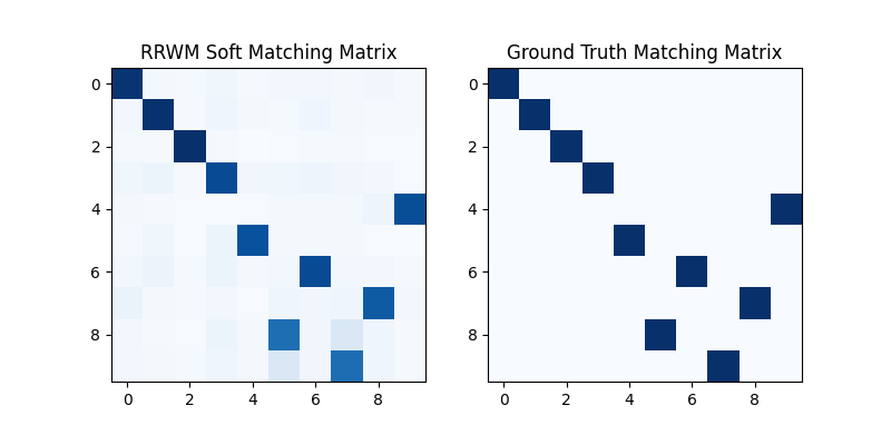
The output of RRWM is a soft matching matrix. The matching prior is well-preserved:

plt.figure(figsize=(8, 4))
plt.subplot(1, 2, 1)
plt.title('RRWM Soft Matching Matrix')
plt.imshow(X.numpy(), cmap='Blues')
plt.subplot(1, 2, 2)
plt.title('Ground Truth Matching Matrix')
plt.imshow(X_gt.numpy(), cmap='Blues')

<matplotlib.image.AxesImage object at 0x00000221B7671850>

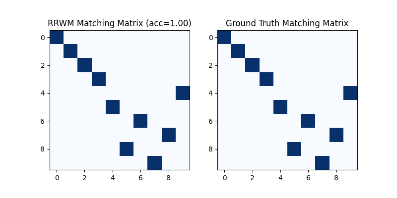
Get the discrete matching matrix

Hungarian algorithm is then adopted to reach a discrete matching matrix

X = pygm.hungarian(X)

Visualization of the discrete matching matrix:

plt.figure(figsize=(8, 4))
plt.subplot(1, 2, 1)
plt.title(f'RRWM Matching Matrix (acc={(X * X_gt).sum()/ X_gt.sum():.2f})')
plt.imshow(X.numpy(), cmap='Blues')
plt.subplot(1, 2, 2)
plt.title('Ground Truth Matching Matrix')
plt.imshow(X_gt.numpy(), cmap='Blues')

<matplotlib.image.AxesImage object at 0x00000221B7E518B0>

Align the original graphs

Draw the matching (green lines for correct matching, red lines for wrong matching, blue lines for seed matching):

plt.figure(figsize=(8, 4))
ax1 = plt.subplot(1, 2, 1)
plt.title('Graph 1')
nx.draw_networkx(G1, pos=pos1)
ax2 = plt.subplot(1, 2, 2)
plt.title('Graph 2')
nx.draw_networkx(G2, pos=pos2)
for i in range(num_nodes):
    j = torch.argmax(X[i]).item()
    if seed_mat[i, j]:
        line_color = "blue"
    elif X_gt[i, j]:
        line_color = "green"
    else:
        line_color = "red"
    con = ConnectionPatch(xyA=pos1[i], xyB=pos2[j], coordsA="data", coordsB="data",
                          axesA=ax1, axesB=ax2, color=line_color)
    plt.gca().add_artist(con)

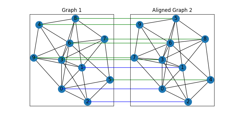
Align the nodes:

align_A2 = torch.mm(torch.mm(X, A2), X.t())
plt.figure(figsize=(8, 4))
ax1 = plt.subplot(1, 2, 1)
plt.title('Graph 1')
nx.draw_networkx(G1, pos=pos1)
ax2 = plt.subplot(1, 2, 2)
plt.title('Aligned Graph 2')
align_pos2 = {}
for i in range(num_nodes):
    j = torch.argmax(X[i]).item()
    align_pos2[j] = pos1[i]
    if seed_mat[i, j]:
        line_color = "blue"
    elif X_gt[i, j]:
        line_color = "green"
    else:
        line_color = "red"
    con = ConnectionPatch(xyA=pos1[i], xyB=align_pos2[j], coordsA="data", coordsB="data",
                          axesA=ax1, axesB=ax2, color=line_color)
    plt.gca().add_artist(con)
nx.draw_networkx(G2, pos=align_pos2)

Other solvers are also available

Only the affinity matrix is modified to encode matching priors, thus other graph matching solvers are also available to handle this seeded graph matching setting.

Classic IPFP solver

See ipfp() for the API reference.

X = pygm.ipfp(K, n1, n2)

Visualization of IPFP matching result:

plt.figure(figsize=(8, 4))
plt.subplot(1, 2, 1)
plt.title(f'IPFP Matching Matrix (acc={(X * X_gt).sum()/ X_gt.sum():.2f})')
plt.imshow(X.numpy(), cmap='Blues')
plt.subplot(1, 2, 2)
plt.title('Ground Truth Matching Matrix')
plt.imshow(X_gt.numpy(), cmap='Blues')

<matplotlib.image.AxesImage object at 0x00000221B7ED0C10>

Classic SM solver

See sm() for the API reference.

X = pygm.sm(K, n1, n2)
X = pygm.hungarian(X)

Visualization of SM matching result:

plt.figure(figsize=(8, 4))
plt.subplot(1, 2, 1)
plt.title(f'SM Matching Matrix (acc={(X * X_gt).sum()/ X_gt.sum():.2f})')
plt.imshow(X.numpy(), cmap='Blues')
plt.subplot(1, 2, 2)
plt.title('Ground Truth Matching Matrix')
plt.imshow(X_gt.numpy(), cmap='Blues')

<matplotlib.image.AxesImage object at 0x00000221B7F878E0>

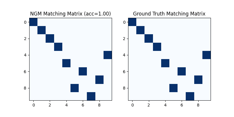
NGM neural network solver

See ngm() for the API reference.

with torch.set_grad_enabled(False):
    X = pygm.ngm(K, n1, n2, pretrain='voc')
    X = pygm.hungarian(X)

Visualization of NGM matching result:

plt.figure(figsize=(8, 4))
plt.subplot(1, 2, 1)
plt.title(f'NGM Matching Matrix (acc={(X * X_gt).sum()/ X_gt.sum():.2f})')
plt.imshow(X.numpy(), cmap='Blues')
plt.subplot(1, 2, 2)
plt.title('Ground Truth Matching Matrix')
plt.imshow(X_gt.numpy(), cmap='Blues')

<matplotlib.image.AxesImage object at 0x00000221B834E9D0>