PyTorch Backend Example: Matching Image Keypoints by QAP Solvers

This example shows how to match image keypoints by graph matching solvers provided by pygmtools. These solvers follow the Quadratic Assignment Problem formulation and can generally work out-of-box. The matched images can be further processed for other downstream tasks.

# Author: Runzhong Wang <runzhong.wang@sjtu.edu.cn>
#
# License: Mulan PSL v2 License

Note

The following solvers support QAP formulation, and are included in this example:

• rrwm() (classic solver)

• ipfp() (classic solver)

• sm() (classic solver)

• ngm() (neural network solver)

import torch # pytorch backend
import torchvision # CV models
import pygmtools as pygm
import matplotlib.pyplot as plt # for plotting
from matplotlib.patches import ConnectionPatch # for plotting matching result
import scipy.io as sio # for loading .mat file
import scipy.spatial as spa # for Delaunay triangulation
from sklearn.decomposition import PCA as PCAdimReduc
import itertools
import numpy as np
from PIL import Image
pygm.set_backend('pytorch') # set default backend for pygmtools

Load the images

Images are from the Willow Object Class dataset (this dataset also available with the Benchmark of pygmtools, see WillowObject).

The images are resized to 256x256.

obj_resize = (256, 256)
img1 = Image.open('../data/willow_duck_0001.png')
img2 = Image.open('../data/willow_duck_0002.png')
kpts1 = torch.tensor(sio.loadmat('../data/willow_duck_0001.mat')['pts_coord'])
kpts2 = torch.tensor(sio.loadmat('../data/willow_duck_0002.mat')['pts_coord'])
kpts1[0] = kpts1[0] * obj_resize[0] / img1.size[0]
kpts1[1] = kpts1[1] * obj_resize[1] / img1.size[1]
kpts2[0] = kpts2[0] * obj_resize[0] / img2.size[0]
kpts2[1] = kpts2[1] * obj_resize[1] / img2.size[1]
img1 = img1.resize(obj_resize, resample=Image.BILINEAR)
img2 = img2.resize(obj_resize, resample=Image.BILINEAR)

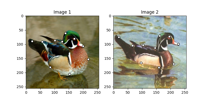
Visualize the images and keypoints

def plot_image_with_graph(img, kpt, A=None):
    plt.imshow(img)
    plt.scatter(kpt[0], kpt[1], c='w', edgecolors='k')
    if A is not None:
        for idx in torch.nonzero(A, as_tuple=False):
            plt.plot((kpt[0, idx[0]], kpt[0, idx[1]]), (kpt[1, idx[0]], kpt[1, idx[1]]), 'k-')

plt.figure(figsize=(8, 4))
plt.subplot(1, 2, 1)
plt.title('Image 1')
plot_image_with_graph(img1, kpts1)
plt.subplot(1, 2, 2)
plt.title('Image 2')
plot_image_with_graph(img2, kpts2)

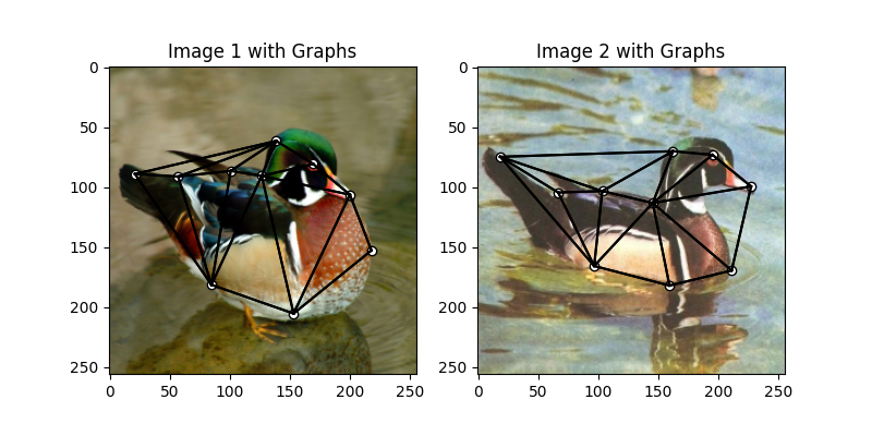
Build the graphs

Graph structures are built based on the geometric structure of the keypoint set. In this example, we refer to Delaunay triangulation.

def delaunay_triangulation(kpt):
    d = spa.Delaunay(kpt.numpy().transpose())
    A = torch.zeros(len(kpt[0]), len(kpt[0]))
    for simplex in d.simplices:
        for pair in itertools.permutations(simplex, 2):
            A[pair] = 1
    return A

A1 = delaunay_triangulation(kpts1)
A2 = delaunay_triangulation(kpts2)

We encode the length of edges as edge features

A1 = ((kpts1.unsqueeze(1) - kpts1.unsqueeze(2)) ** 2).sum(dim=0) * A1
A1 = (A1 / A1.max()).to(dtype=torch.float32)
A2 = ((kpts2.unsqueeze(1) - kpts2.unsqueeze(2)) ** 2).sum(dim=0) * A2
A2 = (A2 / A2.max()).to(dtype=torch.float32)

Visualize the graphs

plt.figure(figsize=(8, 4))
plt.subplot(1, 2, 1)
plt.title('Image 1 with Graphs')
plot_image_with_graph(img1, kpts1, A1)
plt.subplot(1, 2, 2)
plt.title('Image 2 with Graphs')
plot_image_with_graph(img2, kpts2, A2)

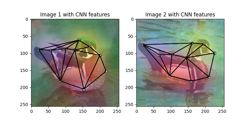
Extract node features

Let’s adopt the VGG16 CNN model to extract node features.

vgg16_cnn = torchvision.models.vgg16_bn(True)
torch_img1 = torch.from_numpy(np.array(img1, dtype=np.float32) / 256).permute(2, 0, 1).unsqueeze(0) # shape: BxCxHxW
torch_img2 = torch.from_numpy(np.array(img2, dtype=np.float32) / 256).permute(2, 0, 1).unsqueeze(0) # shape: BxCxHxW
with torch.set_grad_enabled(False):
    feat1 = vgg16_cnn.features(torch_img1)
    feat2 = vgg16_cnn.features(torch_img2)

Normalize the features

num_features = feat1.shape[1]
def l2norm(node_feat):
    return torch.nn.functional.local_response_norm(
        node_feat, node_feat.shape[1] * 2, alpha=node_feat.shape[1] * 2, beta=0.5, k=0)

feat1 = l2norm(feat1)
feat2 = l2norm(feat2)

Up-sample the features to the original image size

feat1_upsample = torch.nn.functional.interpolate(feat1, (obj_resize[1], obj_resize[0]), mode='bilinear')
feat2_upsample = torch.nn.functional.interpolate(feat2, (obj_resize[1], obj_resize[0]), mode='bilinear')

Visualize the extracted CNN feature (dimensionality reduction via principle component analysis)

pca_dim_reduc = PCAdimReduc(n_components=3, whiten=True)
feat_dim_reduc = pca_dim_reduc.fit_transform(
    np.concatenate((
        feat1_upsample.permute(0, 2, 3, 1).reshape(-1, num_features).numpy(),
        feat2_upsample.permute(0, 2, 3, 1).reshape(-1, num_features).numpy()
    ), axis=0)
)
feat_dim_reduc = feat_dim_reduc / np.max(np.abs(feat_dim_reduc), axis=0, keepdims=True) / 2 + 0.5
feat1_dim_reduc = feat_dim_reduc[:obj_resize[0] * obj_resize[1], :]
feat2_dim_reduc = feat_dim_reduc[obj_resize[0] * obj_resize[1]:, :]

plt.figure(figsize=(8, 4))
plt.subplot(1, 2, 1)
plt.title('Image 1 with CNN features')
plot_image_with_graph(img1, kpts1, A1)
plt.imshow(feat1_dim_reduc.reshape(obj_resize[1], obj_resize[0], 3), alpha=0.5)
plt.subplot(1, 2, 2)
plt.title('Image 2 with CNN features')
plot_image_with_graph(img2, kpts2, A2)
plt.imshow(feat2_dim_reduc.reshape(obj_resize[1], obj_resize[0], 3), alpha=0.5)

<matplotlib.image.AxesImage object at 0x7fd85c402770>

Extract node features by nearest interpolation

rounded_kpts1 = torch.round(kpts1).to(dtype=torch.long)
rounded_kpts2 = torch.round(kpts2).to(dtype=torch.long)
node1 = feat1_upsample[0, :, rounded_kpts1[1], rounded_kpts1[0]].t() # shape: NxC
node2 = feat2_upsample[0, :, rounded_kpts2[1], rounded_kpts2[0]].t() # shape: NxC

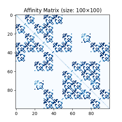
Build affinity matrix

We follow the formulation of Quadratic Assignment Problem (QAP):

\[\begin{split}&\max_{\mathbf{X}} \ \texttt{vec}(\mathbf{X})^\top \mathbf{K} \texttt{vec}(\mathbf{X})\\ s.t. \quad &\mathbf{X} \in \{0, 1\}^{n_1\times n_2}, \ \mathbf{X}\mathbf{1} = \mathbf{1}, \ \mathbf{X}^\top\mathbf{1} \leq \mathbf{1}\end{split}\]

where the first step is to build the affinity matrix (\(\mathbf{K}\))

conn1, edge1 = pygm.utils.dense_to_sparse(A1)
conn2, edge2 = pygm.utils.dense_to_sparse(A2)
import functools
gaussian_aff = functools.partial(pygm.utils.gaussian_aff_fn, sigma=1) # set affinity function
K = pygm.utils.build_aff_mat(node1, edge1, conn1, node2, edge2, conn2, edge_aff_fn=gaussian_aff)

Visualization of the affinity matrix. For graph matching problem with \(N\) nodes, the affinity matrix has \(N^2\times N^2\) elements because there are \(N^2\) edges in each graph.

Note

The diagonal elements are node affinities, the off-diagonal elements are edge features.

plt.figure(figsize=(4, 4))
plt.title(f'Affinity Matrix (size: {K.shape[0]}$\\times${K.shape[1]})')
plt.imshow(K.numpy(), cmap='Blues')

<matplotlib.image.AxesImage object at 0x7fd85c4625f0>

Solve graph matching problem by RRWM solver

See rrwm() for the API reference.

X = pygm.rrwm(K, kpts1.shape[1], kpts2.shape[1])

The output of RRWM is a soft matching matrix. Hungarian algorithm is then adopted to reach a discrete matching matrix.

X = pygm.hungarian(X)

Plot the matching

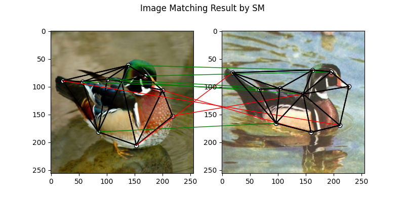
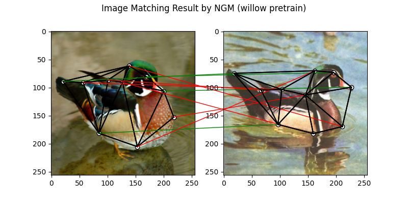
The correct matchings are marked by green, and wrong matchings are marked by red. In this example, the nodes are ordered by their ground truth classes (i.e. the ground truth matching matrix is a diagonal matrix).

plt.figure(figsize=(8, 4))
plt.suptitle('Image Matching Result by RRWM')
ax1 = plt.subplot(1, 2, 1)
plot_image_with_graph(img1, kpts1, A1)
ax2 = plt.subplot(1, 2, 2)
plot_image_with_graph(img2, kpts2, A2)
for i in range(X.shape[0]):
    j = torch.argmax(X[i]).item()
    con = ConnectionPatch(xyA=kpts1[:, i], xyB=kpts2[:, j], coordsA="data", coordsB="data",
                          axesA=ax1, axesB=ax2, color="red" if i != j else "green")
    plt.gca().add_artist(con)

Solve by other solvers

We could also do a quick benchmarking of other solvers on this specific problem.

IPFP solver

See ipfp() for the API reference.

X = pygm.ipfp(K, kpts1.shape[1], kpts2.shape[1])

plt.figure(figsize=(8, 4))
plt.suptitle('Image Matching Result by IPFP')
ax1 = plt.subplot(1, 2, 1)
plot_image_with_graph(img1, kpts1, A1)
ax2 = plt.subplot(1, 2, 2)
plot_image_with_graph(img2, kpts2, A2)
for i in range(X.shape[0]):
    j = torch.argmax(X[i]).item()
    con = ConnectionPatch(xyA=kpts1[:, i], xyB=kpts2[:, j], coordsA="data", coordsB="data",
                          axesA=ax1, axesB=ax2, color="red" if i != j else "green")
    plt.gca().add_artist(con)

SM solver

See sm() for the API reference.

X = pygm.sm(K, kpts1.shape[1], kpts2.shape[1])
X = pygm.hungarian(X)

plt.figure(figsize=(8, 4))
plt.suptitle('Image Matching Result by SM')
ax1 = plt.subplot(1, 2, 1)
plot_image_with_graph(img1, kpts1, A1)
ax2 = plt.subplot(1, 2, 2)
plot_image_with_graph(img2, kpts2, A2)
for i in range(X.shape[0]):
    j = torch.argmax(X[i]).item()
    con = ConnectionPatch(xyA=kpts1[:, i], xyB=kpts2[:, j], coordsA="data", coordsB="data",
                          axesA=ax1, axesB=ax2, color="red" if i != j else "green")
    plt.gca().add_artist(con)

NGM solver

See ngm() for the API reference.

Note

The NGM solvers are pretrained on a different problem setting, so their performance may seem inferior. To improve their performance, you may change the way of building affinity matrices, or try finetuning NGM on the new problem.

The NGM solver pretrained on Willow dataset:

X = pygm.ngm(K, kpts1.shape[1], kpts2.shape[1], pretrain='willow')
X = pygm.hungarian(X)

plt.figure(figsize=(8, 4))
plt.suptitle('Image Matching Result by NGM (willow pretrain)')
ax1 = plt.subplot(1, 2, 1)
plot_image_with_graph(img1, kpts1, A1)
ax2 = plt.subplot(1, 2, 2)
plot_image_with_graph(img2, kpts2, A2)
for i in range(X.shape[0]):
    j = torch.argmax(X[i]).item()
    con = ConnectionPatch(xyA=kpts1[:, i], xyB=kpts2[:, j], coordsA="data", coordsB="data",
                          axesA=ax1, axesB=ax2, color="red" if i != j else "green")
    plt.gca().add_artist(con)

The NGM solver pretrained on VOC dataset:

X = pygm.ngm(K, kpts1.shape[1], kpts2.shape[1], pretrain='voc')
X = pygm.hungarian(X)

plt.figure(figsize=(8, 4))
plt.suptitle('Image Matching Result by NGM (voc pretrain)')
ax1 = plt.subplot(1, 2, 1)
plot_image_with_graph(img1, kpts1, A1)
ax2 = plt.subplot(1, 2, 2)
plot_image_with_graph(img2, kpts2, A2)
for i in range(X.shape[0]):
    j = torch.argmax(X[i]).item()
    con = ConnectionPatch(xyA=kpts1[:, i], xyB=kpts2[:, j], coordsA="data", coordsB="data",
                          axesA=ax1, axesB=ax2, color="red" if i != j else "green")
    plt.gca().add_artist(con)