pygmtools.neural_solvers.ngm
- pygmtools.neural_solvers.ngm(K, n1=None, n2=None, n1max=None, n2max=None, x0=None, gnn_channels=(16, 16, 16), sk_emb=1, sk_max_iter=20, sk_tau=0.05, network=None, return_network=False, pretrain='voc', backend=None)[source]
The NGM (Neural Graph Matching) model for processing the affinity matrix (the most general form of Lawler’s QAP). The math form of graph matching (Lawler’s QAP) is equivalent to a vertex classification problem on the association graph, which is an equivalent formulation based on the affinity matrix \(\mathbf{K}\). The graph matching module is composed of several graph convolution layers, Sinkhorn embedding layers and finally a Sinkhorn layer to output a doubly-stochastic matrix.
See the following pipeline for an example:
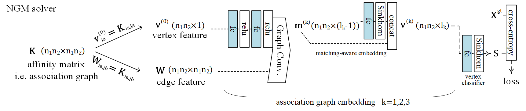
See the following paper for more technical details: “Wang et al. Neural Graph Matching Network: Learning Lawler’s Quadratic Assignment Problem With Extension to Hypergraph and Multiple-Graph Matching. TPAMI 2022.”
- Parameters
K – \((b\times n_1n_2 \times n_1n_2)\) the input affinity matrix, \(b\): batch size.
n1 – \((b)\) number of nodes in graph1 (optional if n1max is given, and all n1=n1max).
n2 – \((b)\) number of nodes in graph2 (optional if n2max is given, and all n2=n2max).
n1max – \((b)\) max number of nodes in graph1 (optional if n1 is given, and n1max=max(n1)).
n2max – \((b)\) max number of nodes in graph2 (optional if n2 is given, and n2max=max(n2)).
x0 – \((b\times n_1 \times n_2)\) an initial matching solution to warm-start the vertex embedding. If not given, the vertex embedding is initialized as a vector of all 1s.
gnn_channels – (default:
(16, 16, 16)) A list/tuple of channel sizes of the GNN. Ignored if the network object is given (ignored ifnetwork!=None)sk_emb – (default: 1) Number of Sinkhorn embedding channels. Sinkhorn embedding is designed to encode the matching constraints inside GNN layers. How it works: a Sinkhorn embedding channel accepts the vertex feature from the current layer and computes a doubly-stochastic matrix, which is then concatenated to the vertex feature. Ignored if the network object is given (ignored if
network!=None)sk_max_iter – (default: 20) Max number of iterations of Sinkhorn. See
sinkhorn()for more details about this argument.sk_tau – (default: 0.05) The temperature parameter of Sinkhorn. See
sinkhorn()for more details about this argument.network – (default: None) The network object. If None, a new network object will be created, and load the model weights specified in
pretrainargument.return_network – (default: False) Return the network object (saving model construction time if calling the model multiple times).
pretrain – (default: ‘voc’) If
network==None, the pretrained model weights to be loaded. Available pretrained weights:voc(on Pascal VOC Keypoint dataset),willow(on Willow Object Class dataset), orFalse(no pretraining).backend – (default:
pygmtools.BACKENDvariable) the backend for computation.
- Returns
if
return_network==False, \((b\times n_1 \times n_2)\) the doubly-stochastic matching matrixif
return_network==True, \((b\times n_1 \times n_2)\) the doubly-stochastic matching matrix, the network object
Note
You may need a proxy to load the pretrained weights if Google drive is not accessible in your contry/region. You may also download the pretrained models manually and put them at
~/.cache/pygmtools(for Linux).Note
This function also supports non-batched input, by ignoring all batch dimensions in the input tensors.
Numpy Example
>>> import numpy as np
>>> import pygmtools as pygm
>>> pygm.set_backend('numpy')
>>> np.random.seed(1)

# Generate a batch of isomorphic graphs
>>> batch_size = 10
>>> X_gt = np.zeros((batch_size, 4, 4))
>>> X_gt[:, np.arange(0, 4, dtype='i4'), np.random.permutation(4)] = 1
>>> A1 = np.random.rand(batch_size, 4, 4)
>>> A2 = np.matmul(np.matmul(X_gt.swapaxes(1, 2), A1), X_gt)
>>> n1 = n2 = np.array([4] * batch_size)

# Build affinity matrix
>>> conn1, edge1, ne1 = pygm.utils.dense_to_sparse(A1)
>>> conn2, edge2, ne2 = pygm.utils.dense_to_sparse(A2)
>>> import functools
>>> gaussian_aff = functools.partial(pygm.utils.gaussian_aff_fn, sigma=1.) # set affinity function
>>> K = pygm.utils.build_aff_mat(None, edge1, conn1, None, edge2, conn2, n1, None, n2, None, edge_aff_fn=gaussian_aff)

# Solve by NGM
>>> X, net = pygm.ngm(K, n1, n2, return_network=True)
Downloading to ~/.cache/pygmtools/ngm_voc_numpy.npy...
>>> (pygm.hungarian(X) * X_gt).sum() / X_gt.sum() # accuracy
1.0

# Pass the net object to avoid rebuilding the model agian
>>> X = pygm.ngm(K, n1, n2, network=net)
>>> (pygm.hungarian(X) * X_gt).sum() / X_gt.sum() # accuracy
1.0

# You may also load other pretrained weights
>>> X, net = pygm.ngm(feat1, feat2, A1, A2, e_feat1, e_feat2, n1, n2, return_network=True, pretrain='willow')
Downloading to ~/.cache/pygmtools/ngm_willow_numpy.npy...
>>> (pygm.hungarian(X) * X_gt).sum() / X_gt.sum() # accuracy
1.0

# You may configure your own model and integrate the model into a deep learning pipeline. For example:
>>> net = pygm.utils.get_network(pygm.ngm, gnn_channels=(32, 64, 128, 64, 32), sk_emb=8, pretrain=False)
# K may be outputs by other neural networks (constructed K from node/edge features by pygm.utils.build_aff_mat)
>>> X = pygm.ngm(K, n1, n2, network=net)
>>> (pygm.hungarian(X) * X_gt).sum() / X_gt.sum() # accuracy
1.0
PyTorch Example
>>> import torch
>>> import pygmtools as pygm
>>> pygm.set_backend('pytorch')
>>> _ = torch.manual_seed(1)

# Generate a batch of isomorphic graphs
>>> batch_size = 10
>>> X_gt = torch.zeros(batch_size, 4, 4)
>>> X_gt[:, torch.arange(0, 4, dtype=torch.int64), torch.randperm(4)] = 1
>>> A1 = torch.rand(batch_size, 4, 4)
>>> A2 = torch.bmm(torch.bmm(X_gt.transpose(1, 2), A1), X_gt)
>>> n1 = n2 = torch.tensor([4] * batch_size)

# Build affinity matrix
>>> conn1, edge1, ne1 = pygm.utils.dense_to_sparse(A1)
>>> conn2, edge2, ne2 = pygm.utils.dense_to_sparse(A2)
>>> import functools
>>> gaussian_aff = functools.partial(pygm.utils.gaussian_aff_fn, sigma=1.) # set affinity function
>>> K = pygm.utils.build_aff_mat(None, edge1, conn1, None, edge2, conn2, n1, None, n2, None, edge_aff_fn=gaussian_aff)

# Solve by NGM
>>> X, net = pygm.ngm(K, n1, n2, return_network=True)
Downloading to ~/.cache/pygmtools/ngm_voc_pytorch.pt...
>>> (pygm.hungarian(X) * X_gt).sum() / X_gt.sum() # accuracy
tensor(1.)

# Pass the net object to avoid rebuilding the model agian
>>> X = pygm.ngm(K, n1, n2, network=net)

# You may also load other pretrained weights
>>> X, net = pygm.ngm(K, n1, n2, return_network=True, pretrain='willow')
Downloading to ~/.cache/pygmtools/ngm_willow_pytorch.pt...

# You may configure your own model and integrate the model into a deep learning pipeline. For example:
>>> net = pygm.utils.get_network(pygm.ngm, gnn_channels=(32, 64, 128, 64, 32), sk_emb=8, pretrain=False)
>>> optimizer = torch.optim.SGD(net.parameters(), lr=0.001, momentum=0.9)
# K may be outputs by other neural networks (constructed K from node/edge features by pygm.utils.build_aff_mat)
>>> X = pygm.ngm(K, n1, n2, network=net)
>>> loss = pygm.utils.permutation_loss(X, X_gt)
>>> loss.backward()
>>> optimizer.step()
Jittor Example
>>> import jittor as jt
>>> import pygmtools as pygm
>>> pygm.set_backend('jittor')
>>> _ = jt.seed(1)

# Generate a batch of isomorphic graphs
>>> batch_size = 10
>>> X_gt = jt.zeros((batch_size, 4, 4))
>>> X_gt[:, jt.arange(0, 4, dtype=jt.int64), jt.randperm(4)] = 1
>>> A1 = jt.rand(batch_size, 4, 4)
>>> A2 = jt.bmm(jt.bmm(X_gt.transpose(1, 2), A1), X_gt)
>>> n1 = n2 = jt.Var([4] * batch_size)

# Build affinity matrix
>>> conn1, edge1, ne1 = pygm.utils.dense_to_sparse(A1)
>>> conn2, edge2, ne2 = pygm.utils.dense_to_sparse(A2)
import functools
>>> gaussian_aff = functools.partial(pygm.utils.gaussian_aff_fn, sigma=1.) # set affinity function
>>> K = pygm.utils.build_aff_mat(None, edge1, conn1, None, edge2, conn2, n1, None, n2, None, edge_aff_fn=gaussian_aff)

# Solve by NGM
>>> X, net = pygm.ngm(K, n1, n2, return_network=True)
# Downloading to ~/.cache/pygmtools/ngm_voc_jittor.pt...
>>> (pygm.hungarian(X) * X_gt).sum() / X_gt.sum() # accuracy
jt.Var([1.], dtype=float32)

# Pass the net object to avoid rebuilding the model agian
>>> X = pygm.ngm(K, n1, n2, network=net)

# You may also load other pretrained weights
>>> X, net = pygm.ngm(K, n1, n2, return_network=True, pretrain='willow')
# Downloading to ~/.cache/pygmtools/ngm_willow_jittor.pt...

# You may configure your own model and integrate the model into a deep learning pipeline. For example:
>>> net = pygm.utils.get_network(pygm.ngm, gnn_channels=(32, 64, 128, 64, 32), sk_emb=8, pretrain=False)
>>> optimizer = jt.optim.SGD(net.parameters(), lr=0.001, momentum=0.9)
# K may be outputs by other neural networks (constructed K from node/edge features by pygm.utils.build_aff_mat)
>>> X = pygm.ngm(K, n1, n2, network=net)
>>> loss = pygm.utils.permutation_loss(X, X_gt)
>>> optimizer.backward(loss)
>>> optimizer.step()
Paddle Example
>>> import paddle
>>> import pygmtools as pygm
>>> pygm.set_backend('paddle')
>>> _ = paddle.seed(1)

# Generate a batch of isomorphic graphs
>>> batch_size = 10
>>> X_gt = paddle.zeros((batch_size, 4, 4))
>>> X_gt[:, paddle.arange(0, 4, dtype=paddle.int64), paddle.randperm(4)] = 1
>>> A1 = paddle.rand((batch_size, 4, 4))
>>> A2 = paddle.bmm(paddle.bmm(X_gt.transpose((0, 2, 1)), A1), X_gt)
>>> n1 = n2 = paddle.to_tensor([4] * batch_size)

# Build affinity matrix
>>> conn1, edge1, ne1 = pygm.utils.dense_to_sparse(A1)
>>> conn2, edge2, ne2 = pygm.utils.dense_to_sparse(A2)
>>> import functools
>>> gaussian_aff = functools.partial(pygm.utils.gaussian_aff_fn, sigma=1.) # set affinity function
>>> K = pygm.utils.build_aff_mat(None, edge1, conn1, None, edge2, conn2, n1, None, n2, None, edge_aff_fn=gaussian_aff)

# Solve by NGM
>>> X, net = pygm.ngm(K, n1, n2, return_network=True)
Downloading to ~/.cache/pygmtools/ngm_voc_paddle.pdparams...
>>> (pygm.hungarian(X) * X_gt).sum() / X_gt.sum() # accuracy
Tensor(shape=[1], dtype=float32, place=Place(cpu), stop_gradient=True,
       [1.])

# Pass the net object to avoid rebuilding the model agian
>>> X = pygm.ngm(K, n1, n2, network=net)

# You may also load other pretrained weights
>>> X, net = pygm.ngm(K, n1, n2, return_network=True, pretrain='willow')
Downloading to ~/.cache/pygmtools/ngm_willow_paddle.pdparams...

# You may configure your own model and integrate the model into a deep learning pipeline. For example:
>>> net = pygm.utils.get_network(pygm.ngm, gnn_channels=(32, 64, 128, 64, 32), sk_emb=8, pretrain=False)
>>> optimizer = paddle.optimizer.SGD(parameters=net.parameters(), learning_rate=0.001)
# K may be outputs by other neural networks (constructed K from node/edge features by pygm.utils.build_aff_mat)
>>> X = pygm.ngm(K, n1, n2, network=net)
>>> loss = pygm.utils.permutation_loss(X, X_gt)
>>> loss.backward()
>>> optimizer.step()
Note
If you find this model useful in your research, please cite:
@ARTICLE{WangPAMI22,
  author={Wang, Runzhong and Yan, Junchi and Yang, Xiaokang},
  journal={IEEE Transactions on Pattern Analysis and Machine Intelligence},
  title={Neural Graph Matching Network: Learning Lawler’s Quadratic Assignment Problem With Extension to Hypergraph and Multiple-Graph Matching},
  year={2022},
  volume={44},
  number={9},
  pages={5261-5279},
  doi={10.1109/TPAMI.2021.3078053}
}